Evaluation on test scenes

This notebook illustrates the use of the L1b CIMR data reader, the retrieval function to write the results to a file. Overall transitioning from the L1b file from the SCEPS or DEIMOS CIMR satellite simulator to a NetCDF file containing the retrieval results.

Note

All code cells are executed when the notebook is run only requiring the source code in the algorithm folder where the reader and algorithm is implemented in the Julia language. In addition a common_functions.jl is used, located in this folder. In this notebook all cells are shown including output from the executed code.

Overview

The multi parameter retrieval was evaluated on the two DEVALGO test cards, as well as on the SCEPS polar test card. For the DEVALGO test cards, the performance is evaluated by analyzing the difference between the retrieval applied to the input brightness temperatures of the CIMR satellite simulator and the retrieval applied to the output of the simulator, i.e., the CIMR L1b data (from DEIMOS). The retrieval is also applied to the SCEPS polar scene where an absolute reference exists in the next section. The brightness temperature before and after the satellite simulator can be used as retrieval input to estimate the effect the CIMR satellite characteristics have on the multi parameter retrieval. In this section, all resampling was performed using a nearest neighbor interpolation. The variables retrieved in the multi parameter retrieval are wind speed WS, total water vapor TWV, cloud liquid water CLW, sea surface temperature SST, ice surface temperature IST, sea ice concentration SIC, multi year ice fraction MYI, first year ice thickness SIT, and sea surface salinity SSS. In the following, the retrieval results are illustrated only for SIC, but the performance metrics are shown for all variables.

Note

The DEVALGO test scenes 1 and 2 contain artificial patterns of different surface types at the geographic location around Svalbard. The geometric pattern shown in this scene, do not correspond to any real scenario and is only for the purpose of testing the retrieval algorithm. The scenes are generated by the DEVALGO team and are not real observations.

Illustration of the reading routines for the data handling

First we are setting up some projection conversion. Since the CIMR L1b data is not on a regular grid, the arrays can not be directly plotted on a map. Therefore, we need to convert the data to a projection that can be plotted on a map.

using Pkg
Pkg.activate("../algorithm/algoenv")
using OEM
using IJulia
using Printf
using Markdown
using Proj
using LinearAlgebra
using NCDatasets
using PythonCall # to call python from julia
using PythonPlot # basically the matplotlib.pyplot module
using Statistics
using Markdown
using OrderedCollections
pygc = pyimport("gc")
pr = pyimport("pyresample")
#cfeature = pyimport("cartopy.feature")
basemap= pyimport("mpl_toolkits.basemap")
LLtoEASE2n = Proj.Transformation("epsg:4326", "epsg:6931")
EASE2NtoLL = inv(LLtoEASE2n)

lltoxy=LLtoEASE2n #conversion from lat/lon to EASE2 grid coordinates
xytoll=EASE2NtoLL #conversion from EASE2 grid coordinates to lat/lon
lea = pr.geometry.AreaDefinition("ease2_nh_testscene","ease2_nh_testscene","ease2_nh_testscene","EPSG:6931",1400,1400,[0,-1.5e6,1.4e6,-1e5]) # uses pyresample to define an area definition for the test region in the EASE2 grid
leaextent=[lea.area_extent[0],lea.area_extent[2],lea.area_extent[1],lea.area_extent[3]] #extent for the image, since order differs from the order in the area definition

#getting the landmask for the region
lealons,lealats=lea.get_lonlats()
landmask = basemap.maskoceans(lealons,lealats,lealats,resolution="i").mask |> PyArray |> Array |> x->.~x 

#defining a cartopy crs
ccrs=lea.to_cartopy_crs()

#can be aceesed like
fns.scene1.l1b

"/DEVALGO/DATA/DEIMOS/W_PT-DME-Lisbon-SAT-CIMR-1B_C_DME_20230420T103323_LD_20280110T114800_20280110T115700_TN.nc"

#the input files can be found on the ESA DEVALGO FTP server,
#this is a named tuple with the paths to the input files
fns = (; scene1=
        (; l1b=joinpath(dpath,"DEIMOS/W_PT-DME-Lisbon-SAT-CIMR-1B_C_DME_20230420T103323_LD_20280110T114800_20280110T115700_TN.nc"),
            input=joinpath(dpath,"DEVALGO/test_scene_1_compressed_lowres.nc")),
        scene2=
        (; l1b=joinpath(dpath,"DEIMOS/W_PT-DME-Lisbon-SAT-CIMR-1B_C_DME_20230417T105425_LD_20280110T114800_20280110T115700_TN.nc"),
            input=joinpath(dpath,"DEVALGO/test_scene_2_compressed_lowres.nc")),
        scenep=
        (;
        l1b = joinpath(dpath,"SCEPS/SCEPS_l1b_sceps_geo_polar_scene_1_unfiltered_tot_minimal_nom_nedt_apc_tot_v2p1.nc"),
        input = joinpath(dpath,"SCEPS/cimr_sceps_toa_card_devalgo_polarscene_1_20161217_v2p0_aa_000.nc"),
        geo = joinpath(dpath,"SCEPS/cimr_sceps_geo_card_devalgo_polarscene_1_20161217_harmonised_v2p0_surface.nc")
        )
)

Simple data reading for a single band can be done with the get_data_for_band function. It only requires the filename of the L1b data and the band to be read. It gets a named tuple with, h, v, lat and lon. All arrays are 1d arrays. h and v are the horizontal and vertical brightness temperatures, lat and lon are the latitude and longitude coordinates. The position in the scan is ignored as the scan direction is already selected by passing “forward” or “backward” to the function. Since this is a raw reader, there is no interpolation or other processing done on the data.

cband_data=get_data_for_band(fns.scene1.l1b,"C_BAND","backward")
@show keys(cband_data) #a named tuple with the keys: h, v, lat, lon,  herr, verr, oza
@show size(cband_data.h);

keys(cband_data) = (:h, :v, :herr, :verr, :lat, :lon, :oza)
size(cband_data.h) = (389932,)

Another possibility is the project_data data function. This also reads a file by name, but also resamples the data onto the closest grid point of the selected band. The output is three arrays with the reprojected brightness temperatures for each band, and the latitude and longitude coordinates of the grid points. The grid points are the same for all bands. The function also takes the scan direction as an argument. The projected brightness temperatures have the different channel as second dimension, starting with the lowest frequency at v pol. The h pol is the next channel, followed by the next higher frequency at v pol and so on, i.e., 10 dimensions in the order L_band_v, L_band_h, C_band_v, C_band_h, X_band_v, X_band_h, Ku_band_v, Ku_band_h, Ka_band_v, Ka_band_h. Here we store forward and backward scans in different arrays, to be able to assess them separately.

Note

The resampling is done by finding the closest grid point in the projection. This is the simplest possible resampling and might not be the best choice for all applications.

Here we fill the arrays with the data from the DEVALGO test scene 1, which is the radiometric scene, with the forward and backward scans in separate arrays, accessed as dictionaries.

band_data=Dict()
band_error=Dict()
latc=Dict()
lonc=Dict()
xc=Dict()
yc=Dict()
for dir in ["forward","backward"]
    band_data[dir],band_error[dir],latc[dir],lonc[dir]=project_data(fns.scene1.l1b,"C_BAND",dir)
    xc[dir],yc[dir]=lltoxy.(latc[dir],lonc[dir]) |> x-> (first.(x),last.(x))
    @eval(@show(size(band_data[$dir])))
    @eval(@show(size(latc[$dir])));
end

size(band_data["forward"]) = (366644, 10)
size(latc["forward"]) = (366644,)

size(band_data["backward"]) = (389932, 10)
size(latc["backward"]) = (389932,)

Illustration of L1b data without resampling

Here it can be seen that the number of data points is different for the different scans. The forward scan contains fewer data points as the calibration is also in forward direction.

Since the data is not on a regular grid, it cannot be plotted directly in the array as it is stored but has to be converted to earth coordinates and possibly resampled. The projection and grid of choice is the EASE2 Northern hemisphere grid. In Fig. 8 is a scatter plot of all the data points of the CIMR L1b data in the EASE2 projection for both viewing directions, forward and backward, is shown individually. For the DEVALGO test scenes, the brightness temperatures outside of the test scene area are 0 K. This is why the data points are only visible in the test scene area. Small structures in the data are visible corresponding to scan lines. Exemplary, only TBh at C-band is shown in Fig. 8.

fig,axs=pyplot.subplots(nrows=2,figsize=(8,8))
for (i,dir) in enumerate(["forward","backward"])
    
    im=i-1 #python indexing starts at 0
    @show size(xc[dir])
    @show size(yc[dir])

    @show size(band_data[dir][:,4])
    img=axs[im].scatter(xc[dir],yc[dir],c=band_data[dir][:,4], vmin=0,vmax=260,s=0.05)
    #img=axs[im].scatter(xc[dir],yc[dir],c=band_error[dir][:,4], vmin=0,vmax=2,s=0.05)
    fig.colorbar(img,ax=axs[im],label="TBh C-band [K]")
    axs[im].set_title(dir*" scan, scene 1")
    axs[im].set_aspect("equal")
    axs[im].set_xlabel("EASE2 North x (km)")
    axs[im].set_ylabel("EASE2 North y (km)")
end
fig.subplots_adjust(hspace=0.3)
plot_with_caption(fig, "C-band TBh forward (upper pane) and backward (lower pane) scans for scene 1.", "scene_scatter")
pyplot.close(fig)
fig=nothing

size(xc[dir]) = (366644,)
size(yc[dir]) = (366644,)
size((band_data[dir])[:, 4]) = (366644,)
size(xc[dir]) = 

(389932,)
size(yc[dir]) = (389932,)
size((band_data[dir])[:, 4]) = (389932,)

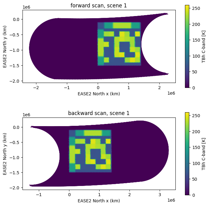
Fig. 8 C-band TBh forward (upper pane) and backward (lower pane) scans for scene 1.

Application of the retrieval on the L1b data

Now we can apply the Multi parameter retrieval using the simple user function run_oem. It takes the band data as produced by the project_data function, i.e., a matrix with (n, 10) dimensions, where n is the number of data points, and 10 is the number of channels. It returns the retrieved parameters similarly as (n, 9) matrix, where the columns are the retrieved parameters. The columns are the same as in the L1b data, i.e., wind speed, total water vapor, cloud liquid water, sea surface temperature, ice surface temperature, sea ice concentration, multi year ice fraction, first year ice thickness, sea surface salinity. The retrieval is done for each scan separately, i.e., the forward and backward scan are retrieved separately.

Index	parameter
1	wind speed [m/s]
2	total water vapor [kg/m²]
3	cloud liquid water [kg/m²]
4	sea surface temperature [K]
5	ice surface temperature [K]
6	sea ice concentration [1]
7	multi year ice fraction [1]
8	first year ice thickness [cm]
9	sea surface salinity [ppt]

The routine also returns the square root of the diagonal of the error covariance matrix of the retrieval and the residuals to the input brightness temperatures, together with the number of iterations.

Here, as an example, we are applying the retrieval to the forward scan and collect the returned variables in a named tuple.

scene1 = Dict()
for dir in ["forward","backward"]
    pygc.collect()
    GC.gc()
    dat,errr,res,its=run_oem(deepcopy(band_data[dir]))#,band_error[dir])
    x,y = xc[dir],yc[dir]; #results from the project_data function above, all still in the scan geometry
    lat,lon = latc[dir],lonc[dir];
    scene1[dir] = (;dat, errr, res, x, y, lat, lon, its) # a named tuple with the results
end

We are providing a cut out of our region of interest, i.e., the location of the test card, in EASE2 projection. This is defined here with the pyresample python package.

lea=pr.geometry.AreaDefinition("ease2_nh_testscene","ease2_nh_testscene","ease2_nh_testscene","EPSG:6931",1400,1400,[0,-1.5e6,1.4e6,-1e5]); #uses pyresample to define an area definition for the test region in the EASE2 grid
leaextent=[lea.area_extent[0],lea.area_extent[2],lea.area_extent[1],lea.area_extent[3]] #extent for the image, since order differs from the order in the area definition

#getting the landmask for the region
lealons,lealats=lea.get_lonlats()
landmask = basemap.maskoceans(lealons,lealats,lealats,resolution="i").mask |> PyArray |> Array |> x->.~x 

#defining a cartopy crs
ccrs=lea.to_cartopy_crs()

<pyresample.utils.cartopy.Projection object at 0x763a5777bad0>

DEVALGO test scene 1 - Radiometric scene

Now we can plot the image of the retrieved parameters, here we chose the sea ice concentration, i.e., index 6. The image is shown in Fig. 9.

let scene1 = scene1["forward"]
    outsic = OEM.project_data_to_area_nn(scene1.dat[:, 6], scene1.lat, scene1.lon, lea)
    fig = pyplot.figure(figsize=(8, 8))
    ax = fig.add_subplot(111, projection=ccrs)
    #outsic[landmask] .= NaN
    ax.imshow(outsic, vmin=0, vmax=1, extent=leaextent, transform=ccrs)

    ax.coastlines(color="red")
    plot_with_caption(fig, "Retrieved SIC on Scene 1 for the forward scan direction.", "scene1_sic_forward")

end

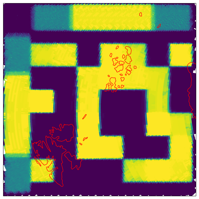
Fig. 9 Retrieved SIC on Scene 1 for the forward scan direction.

Overview of surface classes and true brightness temperatures

For the interpretation of the retrieval results, we can also plot the surface classes. The surface classes were defined in the DEVALGO test cards and were input to several forward models to generate brightness temperatures.

The data for the surface classes is stored in the test scene files. For comparison we can plot the retrieved data on the original input brightness temperature before the CIMR satellite simulator. For test scenes 1 and 2, the helper function read_testscene can be used. It reads the data from the test scenes and returns the brightness temperatures and the pyresample area definition and the image extent. The data block is also a 2d array with the dimensions (n, 10), where n is the number of data points, and 10 is the number of channels. This is to be able to use the same retrieval function for this dataset. The number of data points n is here 1400*1400, i.e., the total number of pixels in the test scene. The area definition is the EASE2 North grid in 1 km resolution. The image extent is the extent of the image in the projection coordinates. This is needed to plot the data on the map.

testinput, mea, imextent, surfaces=read_testscene(fns.scene1.input)

let 
    surface_names=["first year seaice",
    "multi year seaice",
    "snow on land",
    "land without snow",
    "ocean sss=34 SST=275",
    "ocean SSS=6 SST=275",
    "ocean SSS=6 SST=285",
    "ocean SSS=34 SST=285",
    "RFI (5000K)"]

    cmap = matplotlib.cm.get_cmap("viridis", 9)

    fig = pyplot.figure(figsize=(10,8))
    ax = fig.add_subplot(111, projection=ccrs)
    im=ax.imshow(surfaces[end:-1:1,:], extent=imextent, cmap=cmap,interpolation="nearest",vmin=0.5,vmax=9.5)

    cbar_ax = fig.add_axes([0.85, 0.15, 0.04, 0.65])

    cbar = fig.colorbar(im, cax=cbar_ax, ticks=1:9, orientation="vertical")
    #now only show the range 0.5 to 9.5 area of the colorbar, so the surface names are centered for each color and there is no unused color
    cbar.set_ticks(1:9)
    cbar.ax.set_yticklabels(surface_names)

    ax.coastlines()
    plot_with_caption(fig, "Illustration of surface types for scene 1.", "scene1_surfaces")
end

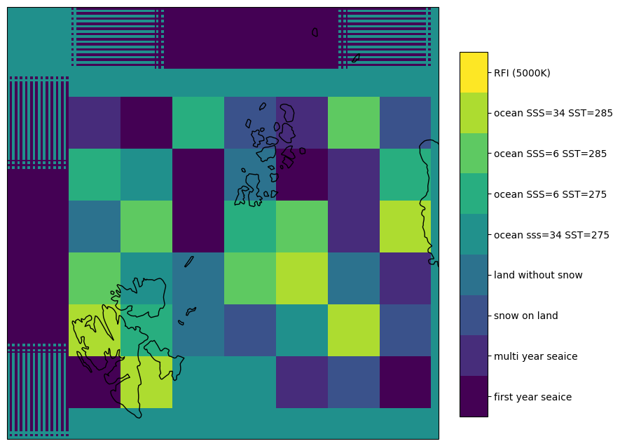
Fig. 10 Illustration of surface types for scene 1.

We can plot all retrieved parameters in a single plot. We chose to define the plotting in a function, to reuse it for the backward scan and the other scenes.

"""
    plot_all_params(dat, x, y, swath=true,mask=true,errors=false)

Plot all parameters from the OEM output in a 3x3 grid.
parameter:
* dat: the output of the OEM algorithm (or error)
* swath: if true, plot the data as a scatter plot, if false, project the data 
to the EASE2 grid and plot as an image
* mask: if true, mask the data according to the sea ice concentration
* errors: if :true (or :std or stderr), plot the error data instead of the data, changing the color scale, limits, etc. accordingly
"""
function plot_all_params(data,direction; swath=true,mask=(:sic,),errors=:false,save=false)
    if direction=="combined"
        ldata= let dat=vcat(data["forward"].dat,data["backward"].dat),
             x=vcat(data["forward"].x,data["backward"].x),y=vcat(data["forward"].y,data["backward"].y),lat=vcat(data["forward"].lat,data["backward"].lat),lon=vcat(data["forward"].lon,data["backward"].lon),errr=vcat(data["forward"].errr,data["backward"].errr),its=vcat(data["forward"].its,data["backward"].its)
            (;dat,x,y,lat,lon,errr,its) |> deepcopy
        end
    else
        ldata=data[direction] |> deepcopy
    end


    
    lealons,lealats=lea.get_lonlats()
    landmask = basemap.maskoceans(lealons,lealats,lealats,resolution="i").mask |> PyArray |> Array |> x->.~x 

    ccrs=lea.to_cartopy_crs()


    fig, ax = pyplot.subplots(nrows=3, ncols=3, figsize=[15, 15], subplot_kw=PyDict(Dict("projection" => ccrs)))
    ax = pyconvert(Array, ax)
    x=ldata.x
    y=ldata.y
    lat=ldata.lat
    lon=ldata.lon
    if errors in (:true,:std,:stderr)
        dat = ldata.errr
        mins = [0, 0, 0, 0, 0, 0, 0, 0, 0]
        #maxs = [10, 10, 0.5, 10, 10, 0.3, 0.3, 100, 5]
        maxs = diag(sqrt.(OEM.S_p))'

        labs = ["wind speed error [m/s]", "total water vapor error [kg/m²]", "cloud liquid water error [kg/m²]",
            "sea surface temperature error [K]", "ice surface temperature error [K]", "sea ice concentration error [1]",
            "multi year ice fraction error [1]", "first year ice thickness error [cm]", "sea surface salinity error [ppt]"]
    elseif errors==:ratio
        dat =  1.0 .- (ldata.errr ./ diag(sqrt.(OEM.S_p))')
        mins = zeros(9)
        maxs = ones(9)
        labs = ["wind speed uncertainty ratio", "total water vapor uncertainty ratio", "cloud liquid water uncertainty ratio",
            "sea surface temperature uncertainty ratio", "ice surface temperature uncertainty ratio", "sea ice concentration uncertainty ratio",
            "multi year ice fraction uncertainty ratio", "first year ice thickness uncertainty ratio", "sea surface salinity uncertainty ratio"]
    elseif errors==:false    
        dat = ldata.dat
        mins = [0, 0, 0, 250, 250, 0, 0, 0, 25]
        maxs = [20, 20, 0.5, 280, 280, 1, 1, 150, 40]
        labs = ["wind speed [m/s]", "total water vapor [kg/m²]", "cloud liquid water [kg/m²]",
        "sea surface temperature [K]", "ice surface temperature [K]", "sea ice concentration [1]",
        "multi year ice fraction [1]", "first year ice thickness [cm]", "sea surface salinity [ppt]"]
    end
    
    cm=pyplot.cm.viridis
    cm.set_bad("grey")
    
    if :sic ∈ mask
        sic=ldata.dat[:,6] #sea ice concentration from original data input, independent if errors is set or not
        dat[sic.>0.9,1].=NaN
        dat[sic.>0.9,4].=NaN
        dat[sic.<0.1,5].=NaN
        dat[sic.<0.1,7].=NaN
        dat[sic.<0.1,8].=NaN
        dat[sic.>0.9,9].=NaN
    end


    for i = 1:9
        if swath
            pos = ax[i].scatter(x, y, c=dat[:, i], s=0.8, vmin=mins[i], vmax=maxs[i])
        else
            cimg = project_data_to_area_nn(dat[:, i], lat, lon, lea)
            cimg = reshape(cimg, 1400, 1400)
            leaextent = [lea.area_extent[0], lea.area_extent[2], lea.area_extent[1], lea.area_extent[3]]
            if :land ∈ mask
                cimg[landmask] .= NaN
            end
            pos = ax[i].imshow(cimg, zorder=1, extent=leaextent, vmin=mins[i], vmax=maxs[i], origin="upper",cmap=cm)
        end
        ax[i].set_title(labs[i])
        cb = fig.colorbar(pos, ax=ax[i], shrink=0.7, orientation="vertical", pad=0.01)
        ax[i].coastlines()
    end
    pyplot.subplots_adjust(wspace=0.01, hspace=0.01)

    if save!=false
        pyplot.savefig(save,dpi=200,bbox_inches="tight")
    end

    return fig
end

Retrieval before and after the satellite simulator for the radiometric scene

Plotting the results resampled to the surface grid 1 km EASE2 North in Fig. 11. The scan lines are barely visible. In this plot the sea ice concentration defines the mask for the other parameters. Wind speed, sea surface temperature and sea surface salinity are shown for small sea ice concentrations while ice surface temperature, sea ice thickness and multi year ice fraction are shown only for higher sea ice concentrations. The total water vapor and cloud liquid water are shown for all sea ice concentrations.

let dir = "forward"
    fig=plot_all_params(scene1,dir,swath=false,mask=(:sic,),errors=:false)
    plot_with_caption(fig, "Retrieved parameters for scene 1 in the forward scan direction.", "scene1_params_forward")
end

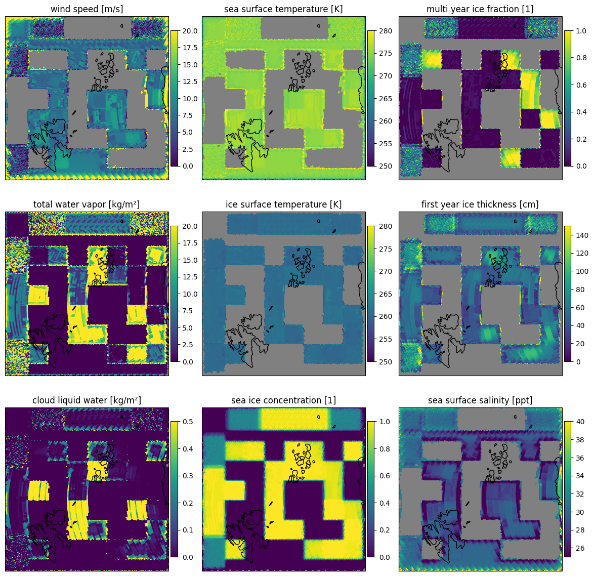
Fig. 11 Retrieved parameters for scene 1 in the forward scan direction.

Despite the forward model not including land surfaces, the retrieval is also run over the land surfaces brightness temperatures, since they are similar to the sea ice brightness temperatures.

The uncertainties are the square root of the diagonal of the error covariance for the retrieved state and are displayed in Fig. 12. From the uncertainties it can be seen that the forward model is not really able to reproduce the brightness temperatures over land surfaces. The uncertainties are very high for the land surfaces, in particular in the cloud liquid water and total water vapor retrieval. The sea ice concentration shows the lowest uncertainties as the sensitivity of the forward model is highest for this parameter. For multi year ice areas which are also retrieved as high multi year ice fraction, the uncertainty of the first year ice thickness retrieval is high as there is little first year ice present.

let dir = "forward"
    fig=plot_all_params(scene1,dir,swath=false,mask=(:sic,),errors=:std)
    plot_with_caption(fig, "Uncertainty after the retrieval for scene 1 in the forward scan direction.", "scene1_params_forward_errors")
end

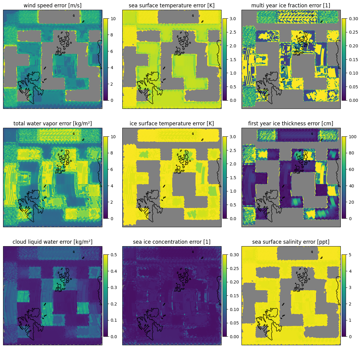
Fig. 12 Uncertainty after the retrieval for scene 1 in the forward scan direction.

In addition to the uncertainty of the retrieval in this Bayesian method, the gained knowledge of the parameters can be assessed. In Fig. 13 we use the 1-uncertainty ratio as a measure of how much our knowledge of each parameter is improved by doing the retrieval, compared to prior knowledge.

Note

The 1-uncertainty ratio (in words: one minus uncertainty ratio) is calculated as the ratio of the prior uncertainty to the posterior uncertainty. A value of 0 means that the retrieval did not improve the knowledge of the parameter, a value of 1 means that the retrieval greatly improved the knowledge of the parameter. As a consequence, this gain in knowledge depends strongly on the prior knowledge of the parameter.

let dir = "forward"
    fig=plot_all_params(scene1,dir,swath=false,mask=(:sic,),errors=:ratio)
    plot_with_caption(fig, "One minus uncertainty ratio before and after th eretrieval for scene 1 in the forward scan direction. 0 means no knowledge improvement, 1 means large knowlege improvement.", "scene1_params_forward_errors_ratio")
end

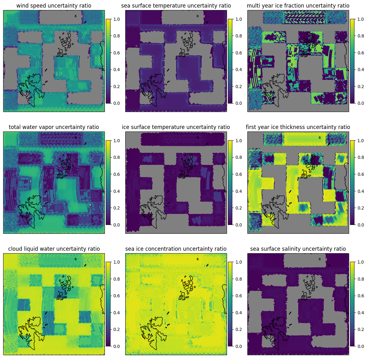
Fig. 13 One minus uncertainty ratio before and after th eretrieval for scene 1 in the forward scan direction. 0 means no knowledge improvement, 1 means large knowlege improvement.

We also apply the retrieval directly to the input data now.

gdata1 = let
    tdat,terr,tres=run_oem(deepcopy(testinput))
    NamedTuple{(:ws, :twv, :clw, :sst, :ist, :sic, :myi, :sit, :sss)}(reshape(tdat[:,i],1400,1400)[end:-1:1,:] for i in 1:9)
end
;

Now we are comparing the retrieved sea ice concentration from the CIMR L1b simulated data to the sea ice concentration retrieved from the input data (to the simulator) in Fig. 14. The difference is very small, which is expected as the simulator is only modifying the input brightness temperature according to the CIMR instrument geometry. The difference is only visible at the ice edges and at the intermediate ice concentration where slight scan pattern are visible from the simulated L1b data.

let scene1 = scene1["forward"]
    fig = pyplot.figure(figsize=(12, 8))

    ax = fig.add_subplot(131, projection=ccrs)
    ax.set_title("SIC on CIMR input, scene 1")
    im=ax.imshow(gdata1.sic,zorder=1,extent=imextent,vmin=0,vmax=1)
    ax.coastlines(color="red")
    pyplot.colorbar(im,orientation="horizontal",pad=0.01)

    outsic=OEM.project_data_to_area_nn(scene1.dat[:,6],scene1.lat,scene1.lon,lea)
    ax = fig.add_subplot(132, projection=ccrs)
    ax.set_title("SIC on CIMR output, scene 1")
    im=ax.imshow(outsic, vmin=0, vmax=1, extent=leaextent, transform=ccrs)
    ax.coastlines(color="red")
    pyplot.colorbar(im,orientation="horizontal",pad=0.01)

    ax = fig.add_subplot(133, projection=ccrs)
    ax.set_title("difference")
    im=ax.imshow(outsic.-gdata1.sic, vmin=-0.3, vmax=0.3, extent=leaextent, transform=ccrs,cmap="RdBu_r")
    pyplot.colorbar(im,orientation="horizontal",pad=0.01)

    ax.coastlines(color="gray")
    plot_with_caption(fig, "Comparison of SIC on CIMR input and output brightness temperatures for scene 1 in forward direction", "scene1_sic_comparison")
end

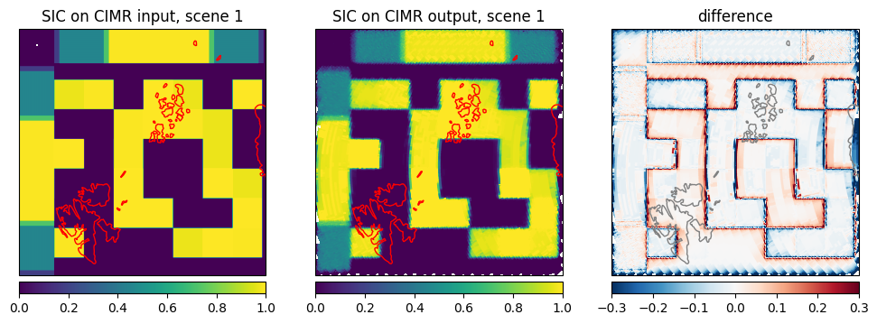
Fig. 14 Comparison of SIC on CIMR input and output brightness temperatures for scene 1 in forward direction

Performance metrics for the radiometric scene

Now we can also calculate the difference between all parameters of the retrieval from the L1b data and the input data. For this we define a helper function to calculate the difference between the retrieval on the input TB and L1b simulation output. Little differences are expected originating only from the satellite simulator edge effects.

"""
calculate_overall_performance(scenes,gdatas,scene_labels,borders)
calculates the overall performance of several scenes and returns an array of values. If direction is set to "combined" it combines the forward and backward retrieval during the reprojection.
scenes is just a array of scenes, gdatas is an array of the truths for corresponding to the scenes
"""
function calculate_overall_performances(scenes,gdatas,directions,borders)
    thevars= ["ws","twv","clw","sst","ist","sic","myi","sit","sss"]
    for direction in directions 
        @assert direction in ["forward","backward","combined"]
    end

    @assert length(scenes)==length(gdatas)==length(borders)
    results=OrderedDict()
    for j in axes(thevars,1)
        results[thevars[j]]=OrderedDict()
        for direction in directions
            diffs = []
            truthes = []
            for i in axes(scenes,1)
                if direction=="combined"
                    cimg = project_data_to_area_nn([scenes[i]["forward"].dat[:, j]; scenes[i]["backward"].dat[:,j]], [scenes[i]["forward"].lat; scenes[i]["backward"].lat], [scenes[i]["forward"].lon; scenes[i]["backward"].lon], lea)
                else
                    cimg = project_data_to_area_nn(scenes[i][direction].dat[:, j], scenes[i][direction].lat, scenes[i][direction].lon, lea)
                end
                cimg = reshape(cimg, 1400, 1400)
                cimg_ref=gdatas[i][Symbol(thevars[j])][:]
                cimg_ref=reshape(cimg_ref,1400,1400)
                diff=cimg.-cimg_ref
                
                diff=diff[borders[i]:end-borders[i],borders[i]:end-borders[i]][:] |> x->filter(!isnan,x)
                push!(diffs,diff)
                push!(truthes,cimg_ref[borders[i]:end-borders[i],borders[i]:end-borders[i]][:] |> x->filter(!isnan,x))
            end
            results[thevars[j]][direction]=(;meanvalue=mean(vcat(truthes...)),mean=mean(vcat(diffs...)),std=std(vcat(diffs...)))
        end
    end
     return results
end

function markdown_table(results,title,label;include_mean=false,show_units=true)
    thevars= ["ws","twv","clw","sst","ist","sic","myi","sit","sss"]
    units=Dict("ws"=>"m/s","twv"=>"kg/m²","clw"=>"kg/m²","sst"=>"K","ist"=>"K","sic"=>"1","myi"=>"1","sit"=>"cm","sss"=>"ppt")
    #create markdown table, MyST markdown if in jupyter book compilation, normal otherwise
    outstring="```{list-table} Performance metric for $title\n"
    outstring *=":name: \"performance-$label\"\n"
    outstring *=":header-rows: 1\n"
    
    directions= results[thevars[1]] |> keys

    sdirs=Dict("forward"=>"fw","backward"=>"bw","combined"=>"cb")
    if get(ENV,"JUPYTER_BOOK_BUILD","false") == "true"
        if include_mean
            outstring *="* - Variable\n "* mapreduce(x->"  - $(sdirs[x]) mean value\n  - $(sdirs[x]) mean(diff)\n  - $(sdirs[x]) std(diff)\n",*,directions)
        else
            outstring *="* - Variable\n "* mapreduce(x->"  - $(sdirs[x]) mean(diff)\n  - $(sdirs[x]) std(diff)\n",*,directions)
        end
        for var in thevars
            vals = results[var]
            if show_units
                outstring *= "* - $(uppercase(var)) [$(units[var])]\n"
            else
                outstring *= "* - $(uppercase(var))\n"
            end
            if include_mean
                outstring *= mapreduce(x->"  - $(@sprintf "%.3f" x.meanvalue)\n  - $(@sprintf "%.3f" x.mean)\n  - $(@sprintf "%.3f" x.std)\n",*,(vals[direction] for direction in directions))
            else
                outstring *= mapreduce(x->"  - $(@sprintf "%.3f" x.mean)\n  - $(@sprintf "%.3f" x.std)\n",*,(vals[direction] for direction in directions)) 
            end
            #outstring *=  (@sprintf "  - %.3f\n  - %.3f\n" vals.mean vals.std)
            #
        end
        outstring *= "```"
    else
        outstring= "~~~markdown\n"*outstring*"\n# table content (skipped in notebook) ```\n~~~\n"
        outstring *="| Variable |"
        if include_mean
            outstring *= mapreduce(x->" $(sdirs[x]) mean value | $(sdirs[x]) mean(diff) | $(sdirs[x]) std(diff) |",*,directions) *"\n"
        else
            outstring *= mapreduce(x->" $(sdirs[x]) mean(diff) | $(sdirs[x]) std(diff) |",*,directions) *"\n"
        end
        #outstring *="| Variable |"*" mean(diff) | std(diff) |"^(length(directions))*"\n"
        if include_mean
            outstring *="| --- "
        end
        outstring *="| --- |"*" --- | --- |"^(length(directions) )*"\n"
        for var in thevars
            vals = results[var]
            if show_units
                outstring *= "| $(uppercase(var)) [$(units[var])] |"
            else
                outstring *= "| $(uppercase(var)) |"
            end
            if include_mean
                outstring *= mapreduce(x->" $(@sprintf "%.3f" x.meanvalue) | $(@sprintf "%.3f" x.mean) | $(@sprintf "%.3f" x.std) |",*,(vals[direction] for direction in directions)) *"\n"
            else
                outstring *= mapreduce(x->" $(@sprintf "%.3f" x.mean) | $(@sprintf "%.3f" x.std) |",*,(vals[direction] for direction in directions)) *"\n"
            end
            #outstring *= "| $(uppercase(var)) | $(@sprintf "%.3f" vals.mean) | $(@sprintf "%.3f" vals.std) |\n"
        end
    end

    return outstring
end

calculate_overall_performances([scene1], [gdata1], ["combined"], [100]) |> x-> markdown_table(x,"scene 1","1",include_mean=true,show_units=true) |> x->display("text/markdown",Markdown.parse(x));

Table 3 Performance metric for scene 1

Variable	cb mean value	cb mean(diff)	cb std(diff)
WS [m/s]	9.189	-1.124	4.896
TWV [kg/m²]	3.286	1.033	11.918
CLW [kg/m²]	-0.023	0.007	0.212
SST [K]	275.082	0.014	1.283
IST [K]	260.380	-0.362	1.302
SIC [1]	0.482	0.003	0.186
MYI [1]	0.253	0.128	0.377
SIT [cm]	81.951	13.787	61.831
SSS [ppt]	30.004	-0.829	2.210

In table Table 3 the mean difference and the root mean square difference between the retrieved parameters from the input data and the L1b data are shown in forward and backward combined scans (cb). The differences are very small as expected. The differences are only visible at the ice edges and at the intermediate ice concentration where slight scan pattern are visible from the simulated L1b data.

DEVALGO test scene 2 - Geometric scene

Retrieval before and after the satellite simulator for the geometric scene

We perform the same comparison for the test scene 2, also for the forward scan. This scene is also called the geometric scene.

#get cimer results
#scene2 = let dir="forward"
scene2 = Dict()
for dir in ["forward","backward"]
    test2datac,test2derror,lat,lon=project_data(fns.scene2.l1b,"C_BAND",dir)
    x,y=lltoxy.(lat,lon) |> x-> (first.(x),last.(x))
    pygc.collect()
    GC.gc()
    dat,err,res=run_oem(deepcopy(test2datac))
    scene2[dir] = (; dat, err, res, x, y, lat, lon)
end

let dir="forward"
    fig=plot_all_params(scene2,dir,swath=false,mask=(:sic,),errors=:false)
    plot_with_caption(fig, "Retrieved parameters for scene 2 in the forward scan direction.", "scene2_params_forward")
end

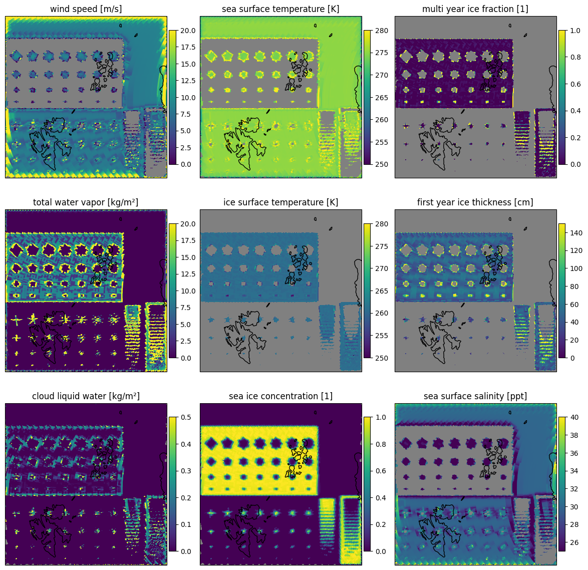
Fig. 15 Retrieved parameters for scene 2 in the forward scan direction.

It can be seen from Fig. 15, that in this test scene, the different shapes and patterns are a major challenge for the retrieval and the smearing introduced by the lower resolution channels is more apparent. For the mask here again only the retrieved ice concentration is used, like before with the radiometric scene.

Then we read again the input and apply the retrieval to that data for comparison.

gdata2 = let
    test2data,lea,imextent,surfaces=read_testscene(fns.scene2.input)
    pygc.collect()
    GC.gc()
    tdat,terr,tres=run_oem(deepcopy(test2data))
    NamedTuple{(:ws, :twv, :clw, :sst, :ist, :sic, :myi, :sit, :sss)}(reshape(tdat[:,i],1400,1400)[end:-1:1,:] for i in 1:9)
end;

We focus on the sea ice concentration also on test scene 2 in Fig. 16. Here again, the difference is rather small and only visible at the edges of the ice, and the edges of the scene.

let scene2 = scene2["forward"]
    fig = pyplot.figure(figsize=(12, 8))
    scene=2
    ax = fig.add_subplot(131, projection=ccrs)
    ax.set_title("SIC on CIMR input, scene $scene")

    im=ax.imshow(gdata2.sic ,zorder=1,extent=imextent,vmin=0,vmax=1)
    ax.coastlines(color="red")
    pyplot.colorbar(im,orientation="horizontal",pad=0.01)

    ax = fig.add_subplot(132, projection=ccrs)
    ax.set_title("SIC on CIMR output, scene $scene")
    outsic=OEM.project_data_to_area_nn(scene2.dat[:,6],scene2.lat,scene2.lon,lea)

    im=ax.imshow(outsic, vmin=0, vmax=1, extent=leaextent, transform=ccrs)
    ax.coastlines(color="red")
    pyplot.colorbar(im,orientation="horizontal",pad=0.01)

    ax = fig.add_subplot(133, projection=ccrs)
    ax.set_title("difference")
    im=ax.imshow(outsic.-gdata2.sic, vmin=-0.3, vmax=0.3, extent=leaextent, transform=ccrs,cmap="RdBu_r")
    pyplot.colorbar(im,orientation="horizontal",pad=0.01)

    ax.coastlines(color="gray")
    plot_with_caption(fig, "SIC on CIMR input, output and difference for scene 2", "SIC_comparison_scene2")
end

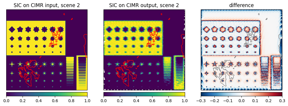
Fig. 16 SIC on CIMR input, output and difference for scene 2

Performance metrics for the geometric scene

Also for this scene we can calculate the performance of the retrieval on the input data and the L1b data. The results are shown in table Table 4. The bias is very small, while the RMSE is similar to the RMSE in the radiometric scene.

calculate_overall_performances([scene2], [gdata2], ["combined"], [100]) |> x-> markdown_table(x,"scene 2","2", include_mean=true ) |> x->display("text/markdown",Markdown.parse(x))

Table 4 Performance metric for scene 2

Variable	cb mean value	cb mean(diff)	cb std(diff)
WS [m/s]	7.208	-0.960	3.977
TWV [kg/m²]	0.746	2.173	14.140
CLW [kg/m²]	-0.110	0.026	0.175
SST [K]	274.980	0.171	1.594
IST [K]	260.253	-0.266	1.490
SIC [1]	0.332	0.007	0.172
MYI [1]	0.196	0.122	0.415
SIT [cm]	84.410	14.630	63.438
SSS [ppt]	29.957	-0.882	2.687

Test scene SCEPS - Polar scene

We perform the same comparison for the SCEPS polar test scene.

Then we read again the input and apply the retrieval to that data for comparison. Since the format of the SCEPS input scene is slightly different, we have another reading routine for this dataset.

data=Dict()
scenep=Dict()
for dir in ["forward","backward"]
    test2datac,test2errorc,lat,lon=project_data(fns.scenep.l1b,"C_BAND",dir,oza_corr=true)
    x,y=lltoxy.(lat,lon) |> x-> (first.(x),last.(x))
    dat,errr,res,its=run_oem(test2datac)
    data[dir]=NamedTuple{(:ws, :twv, :clw, :sst, :ist, :sic, :myi, :sit, :sss)}(OEM.project_data_to_area_nn(dat[:,i],lat,lon,lea) for i in 1:9)
    scenep[dir]=(;dat, errr, res, lat, lon,x,y,its)
end

Here we can discuss the results of the multi parameter retrieval on a the polar scene and give some interpretation of the results. We are lookingn into the combined results from the forward and backward scans. Since we use a simplistic near-neighbour approach, we expect some noise in the results, where the retrieval on the forward and backward scans do not match well. Three different quantities are shown here

• the retrieved parameters Fig. 17

• the uncertainty of the retrieval Fig. 18

• the improvement of our knowledge of the parameters (one minus square root of diagonal of the covariance matrix) Fig. 19

The results are shown in the following plots.

let dir="combined"
    fig=plot_all_params(scenep,dir, swath=false,mask=(:sic,:land),errors=:false)
    description="Retrieval results for the nine parameters for the combined forward and backward scans for the SCEPS polar scene."
    plot_with_caption(fig,description,"retrieval_polar_combined")
end

Fig. 17 Retrieval results for the nine parameters for the combined forward and backward scans for the SCEPS polar scene.

The quantities are reasonable, while some have a bit more noise and others are more stable. The SIC is very smooth with little noise which is expected as it has the highest influence on the brightness temperatures. SSS, IST and SST look flat, as if not the real variability of these variables is preserved. This is due to the fact that the retrieval is not very sensitive to these parameters. The SIC is the most important parameter for the retrieval and the other parameters are more relying on the apri ori data. The uncertainty of the retrieval is quite high for the SSS, IST and SST, while it is low for the SIC. This can be seen when we plot the uncertainty of the retrieval below.

let dir="combined"
    fig=plot_all_params(scenep,dir, swath=false,mask=(:sic,:land),errors=:true)
    description="Retrieval uncertainty for the nine parameters for the combined forward and backward scans for the SCEPS polar scene."
    plot_with_caption(fig,description,"uncertainty_polar_combined")
end

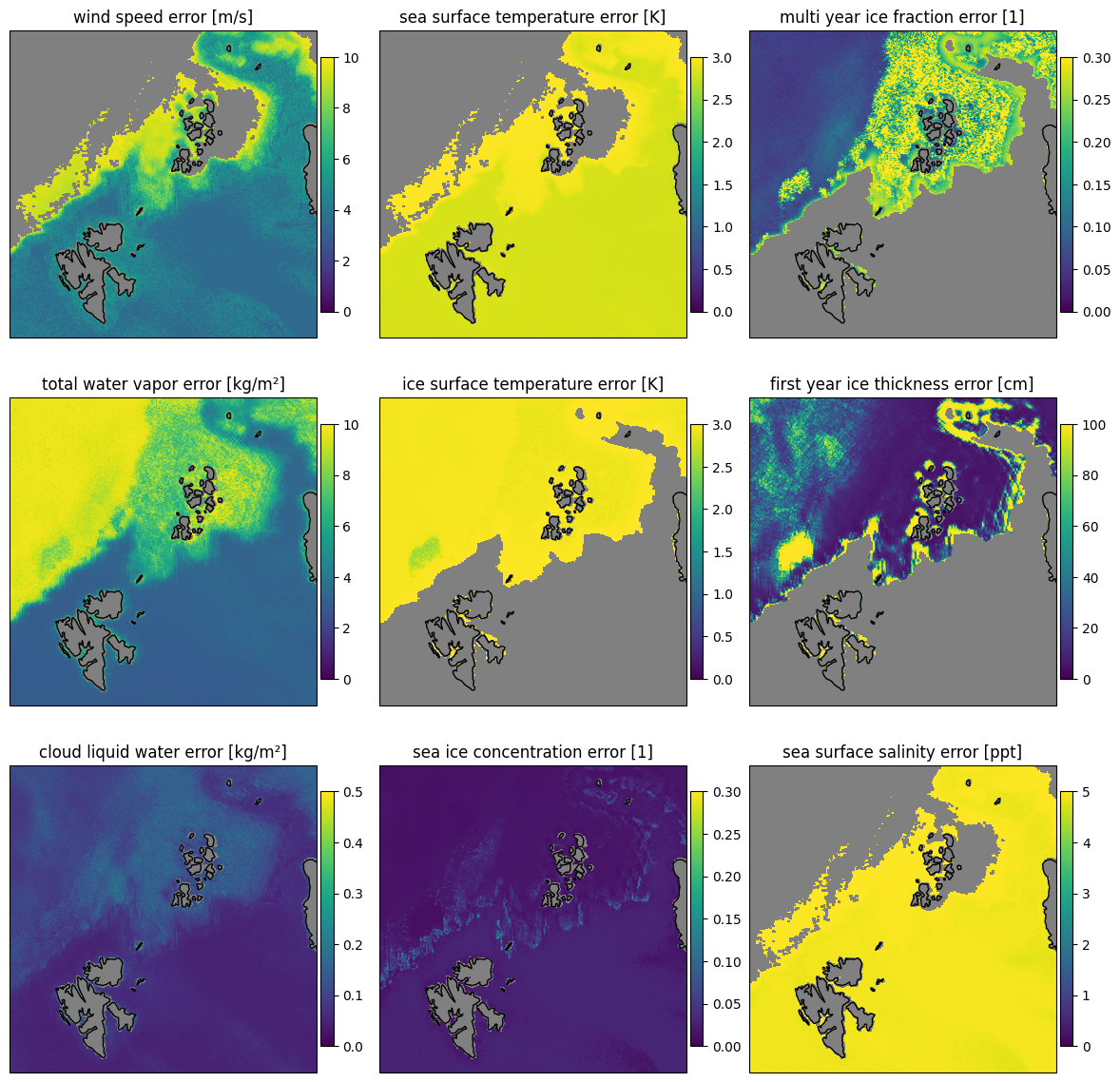
Fig. 18 Retrieval uncertainty for the nine parameters for the combined forward and backward scans for the SCEPS polar scene.

The comparison to the prior uncertainty shows that the retrieval improves our knowledge of the parameters. The improvement is highest for the SIC except over the ice edge, while it is lowest for the IST and SSS as these variables have little influence on the resulting TBs compared to the others. Also the CLW and the SIT was show a good improvement of our knowledge by performing the retrieval.

let dir="combined"
    fig=plot_all_params(scenep,dir, swath=false,mask=(:sic,:land),errors=:ratio)
    description="Retrieval knowledge improvement for the nine parameters for the combined forward and backward scans for the SCEPS polar scene. Zeros means no improvement over prior, while ones means vast improvement."
    plot_with_caption(fig,description,"improvement_polar_combined")
end

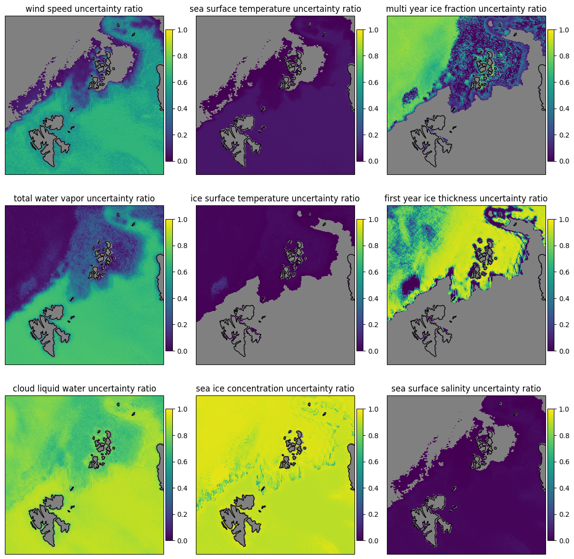
Fig. 19 Retrieval knowledge improvement for the nine parameters for the combined forward and backward scans for the SCEPS polar scene. Zeros means no improvement over prior, while ones means vast improvement.

Next we do a comparison to the retrieval on the input data to the satellite simulator is done. This is done to show that the retrieval is able to retrieve the parameters from the input data. We do not explicitly compare all variables here for the retrieval on input and output data of the simulator.

gdatap = let
    stest,_,imextent=OEM.read_testscene_sceps(fns.scenep.input)
    tdat,terr,tres=run_oem(deepcopy(stest))

    NamedTuple{(:ws, :twv, :clw, :sst, :ist, :sic, :myi, :sit, :sss)}(
        let cdat=reshape(tdat[:,i],1400,1400)|>rotl90 #somehow the data is rotated
            cdat[landmask].=NaN
            cdat
        end for i in 1:9)
end;

As an example, we discuss the SIC from the retrieval and compare between the retrieval applied to the input data and the L1b data. The difference is very small as expected, as the simulator is only adding noise and a smearing of the footprints to the data. The difference is only visible at the ice edges and at the intermediate ice concentration where slight scan pattern are visible from the simulated L1b data.

let fig = pyplot.figure(figsize=(12, 8))
    scene="polar"
    ax = fig.add_subplot(131, projection=ccrs)
    ax.set_title("SIC on CIMR input $scene")
    im=ax.imshow(gdatap.sic,zorder=1,extent=leaextent,vmin=0,vmax=1)
    ax.coastlines(color="red")
    pyplot.colorbar(im,orientation="horizontal",pad=0.01)

    ax = fig.add_subplot(132, projection=ccrs)
    ax.set_title("SIC on CIMR output, scene $scene")

    outsic=data["forward"].sic
    outsic[landmask].=NaN
    im=ax.imshow(outsic, vmin=0, vmax=1, extent=leaextent, transform=ccrs)
    ax.coastlines(color="red")
    pyplot.colorbar(im,orientation="horizontal",pad=0.01)

    ax = fig.add_subplot(133, projection=ccrs)
    ax.set_title("difference")
    im=ax.imshow(data["forward"].sic.-gdatap.sic, vmin=-0.3, vmax=0.3, extent=leaextent, transform=ccrs,cmap="RdBu_r")
    pyplot.colorbar(im,orientation="horizontal",pad=0.01)

    ax.coastlines(color="gray")
    plot_with_caption(fig,"SIC comparison between CIMR input and output for scene $scene, SIC on CIMR input TBs (left), SIC on CIMR output, the L1b (middle), their difference (right)", "SIC_comparison_$scene.png")
end

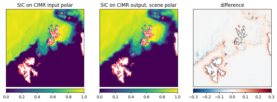
Fig. 20 SIC comparison between CIMR input and output for scene polar, SIC on CIMR input TBs (left), SIC on CIMR output, the L1b (middle), their difference (right)

Analog to the other scenes, we calculate the performance of the retrieval on the input data and the L1b data. The combined results for forward and backward scan are in table Table 5. Here we did not remove the border pixels from the comparison, as the SCEPS polar scene does not have a 0 K border as the other scenes. The table shows the smallest mean difference (bias) in SIC, CLW and MYI, while the other variables also show good performance. The standard deviation of the difference is a measure of how far the results spread around the mean difference. TWV and WS show very high values, but also the SSS and SIT values are quite large. The SIC as the value with the smallest bias, also has very low spread.

calculate_overall_performances([scenep], [gdatap], ["combined"], [1]) |> x-> markdown_table(x,"scene 1","polar-combined") |> x -> display("text/markdown",x) 

Table 5 Performance metric for scene 1

Variable	cb mean(diff)	cb std(diff)
WS [m/s]	-0.155	3.501
TWV [kg/m²]	-0.156	4.588
CLW [kg/m²]	0.003	0.072
SST [K]	-0.196	0.439
IST [K]	-0.000	0.379
SIC [1]	0.007	0.056
MYI [1]	0.006	0.092
SIT [cm]	4.162	18.406
SSS [ppt]	0.092	1.417

We are loading the SCEPS polar scene reference geophysical data for comparison. It is already in EASE2 projection with the same grid as the reference brightness temperatures.

gdata_true,latt,lont = let
     #fn="/home/huntemann/CIMR_L1X/cimr_sceps_geo_card_polarscene_1_20161217_v1p0_part1.nc"
    fn=fns.scenep.geo


    NamedTuple{(:ws, :twv, :clw, :sst, :ist, :sic, :myi, :sit, :sss, :snd, :fdn)}((
    (((NCDataset(fn)["surface_wind_u"][:,:,1]).^2f0
    .+(NCDataset(fn)["surface_wind_v"][:,:,1]).^2f0).^(0.5f0))[end:-1:1,:],
    NCDataset(fn)["total_column_water_vapour"][:,:,1][end:-1:1,:],
    NCDataset(fn)["total_column_liquid_water"][:,:,1][end:-1:1,:],
    NCDataset(fn)["sea_surface_temperature"][:,:,1][end:-1:1,:],
    NCDataset(fn)["sea_ice_temperature"][:,:,1][end:-1:1,:],
    NCDataset(fn)["sea_ice_concentration"][:,:,1][end:-1:1,:]/100.0f0,
    NCDataset(fn)["sea_ice_type"][:,:,1][end:-1:1,:], #1=multiyear, 0=first year (or no ice)
    NCDataset(fn)["sea_ice_thickness"][:,:,1][end:-1:1,:]*100.0f0,
    
    NCDataset(fn)["sea_surface_salinity"][:,:,1][end:-1:1,:],
    NCDataset(fn)["snow_thickness"][:,:,1][end:-1:1,:]*100.0f0,
    NCDataset(fn)["freezing_days_number"][:,:,1][end:-1:1,:]
    )),
    NCDataset(fn)["latitude"][:,:,1][end:-1:1],
    NCDataset(fn)["longitude"][:,:,1][end:-1:1]
end;

Here we get an overview over the reference values of the SCEPS polar scene.

#overview plot of all gdata_true variables 3x3 grid
mmdict=Dict("ws"=>[0,20],"twv"=>[0,20],"clw"=>[0,0.5],"sst"=>[250,280],"ist"=>[250,280],"sic"=>[0,1],"myi"=>[0,1],"sit"=>[0,150],"sss"=>[28,35], "snd"=>[0,50],"fdn"=>[0,100])
#variable names and units
labdict=Dict("ws"=>"wind speed [m/s]","twv"=>"total water vapor [kg/m²]","clw"=>"cloud liquid water [kg/m²]","sst"=>"sea surface temperature [K]","ist"=>"ice surface temperature [K]","sic"=>"sea ice concentration [1]","myi"=>"multi year ice fraction [1]","sit"=>"first year ice thickness [cm]","sss"=>"sea surface salinity [ppt]", "snd"=>"snow thickness [cm]","fdn"=>"freezing days number [1]")

fig,ax=pyplot.subplots(nrows=3,ncols=3,figsize=[15,15],subplot_kw=PyDict(Dict("projection"=> ccrs)))
ax=pyconvert(Array,ax)[:]

for (i,varname) in enumerate(Symbol.(("ws","twv","clw","sst","ist","sic","myi","sit","sss")))
    mins,maxs = mmdict[string(varname)]
    pos=ax[i].imshow(getfield(gdata_true,varname),extent=leaextent,vmin=mins,vmax=maxs,cmap="viridis",transform=ccrs)
    cb=fig.colorbar(pos,ax=ax[i],shrink=0.7,orientation="vertical",pad=0.01)
    ax[i].set_title(labdict[string(varname)])
    #ax[i].set_extent(extent,mycrs)
    ax[i].coastlines()
end
pyplot.subplots_adjust(wspace=0.01,hspace=0.01)
#display("image/png",fig)
plot_with_caption(fig, "SCEPS Polar scene reference geophysical data for the nine variables which are also used in the multi parameter retrieval.", "sceps_polar_reference")

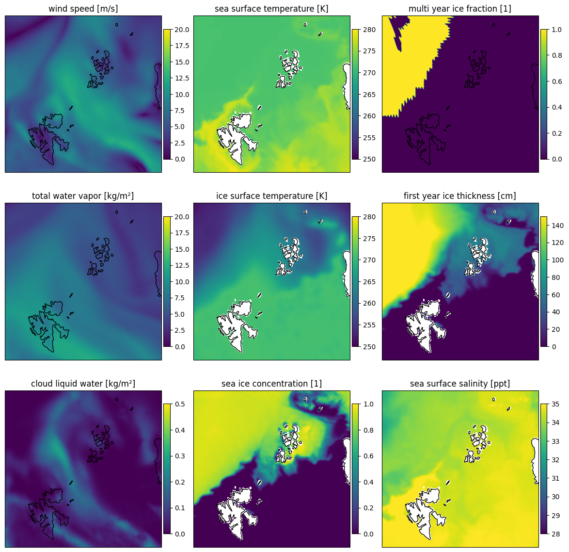
Fig. 21 SCEPS Polar scene reference geophysical data for the nine variables which are also used in the multi parameter retrieval.

Here we perform a comparison of the SCEPS polar scene reference data to the retrieval performed on L1b data.

• Wind Speed (WS): A similar pattern is visible in both datasets. The retrieval shows a little higher values in general (Fig. 22).

• Total Water Vapor (TWV): The pattern is similar, but the retrieval shows lower values in general. The retrieval shows discontinuity over the ice edge (Fig. 23).

• Cloud Liquid Water (CLW): The pattern is similar, also the absolute range of values is similar. The retrieval shows a discontinuity over the ice edge (Fig. 24).

• Sea Surface Temperature (SST): The retrieval seems uniformly retrieving similar values close to the freezing point while the reference data shows more variation and higher temperatures (Fig. 25).

• Ice Surface Temperature (IST): The retrieval shows quite high values around the freezing point uniformly, while the reference data shows much lower temperatures closer towards the North pole (Fig. 26).

• Sea Ice Concentration (SIC): The retrieval shows a similar pattern as the reference data, but lower values at the ice edge (Fig. 27).

• Multi Year Ice Fraction (MYI): The reference data is binary (multiyear ice or not). All multiyear ice according to the reference is retrieved as increased multiyear ice fraction between 0.6 and 1.0, while the first year ice is retrieved as 0.0 as expected (Fig. 28).

• First Year Ice Thickness (SIT): The comparable first year ice area shows similar sea ice thickness, while the retrieval shows slightly lower values in general (Fig. 29).

• Sea Surface Salinity (SSS): The retrieval shows lower values close to the a priori value of 30ppt while the reference data has mostly values around 35ppt (Fig. 30).

#varname="twv"
dir="forward"
for varname in ["ws","twv","clw","sst","ist","sic","myi","sit","sss"]
    mins,maxs = mmdict[varname]
    fig = pyplot.figure(figsize=(12, 4.5))
    scene="polar"
    #fig.suptitle(labdict[varname])

    #left plot
    ax = fig.add_subplot(131, projection=ccrs)
    ax.set_title("$(uppercase(varname)) reference, scene $scene")
    truedat=getfield(gdata_true,Symbol(varname))
    truedat[landmask].=NaN
    im=ax.imshow(truedat, vmin=mins, vmax=maxs, extent=leaextent, transform=ccrs)
    ax.coastlines(color="gray")
    pyplot.colorbar(im,orientation="horizontal",pad=0.01)
   
    #center plot
    ax = fig.add_subplot(132, projection=ccrs)
    ax.set_title("$(uppercase(varname)) on CIMR output, scene $scene")
    retrdat = getfield(data["forward"],Symbol(varname))
    retrdat[landmask].=NaN
    im=ax.imshow(retrdat,zorder=1,extent=leaextent,vmin=mins,vmax=maxs)
    ax.coastlines(color="gray")
    pyplot.colorbar(im,orientation="horizontal",pad=0.01)

    #right plot
    ax = fig.add_subplot(133, projection=ccrs)
    ax.set_title("difference")
    diffs=getfield(gdata_true,Symbol(varname)).-getfield(data[dir],Symbol(varname))
    diffmax=quantile(filter(!isnan,abs.(diffs)[:]) ,0.95)
    im=ax.imshow(diffs, vmin=-diffmax, vmax=diffmax, extent=leaextent, transform=ccrs,cmap="RdBu_r")
    pyplot.colorbar(im,orientation="horizontal",pad=0.01)

    ax.coastlines(color="gray")
    plot_with_caption(fig, "Comparison of $(uppercase(varname)) between reference dataset and retrieval.", "ref_comparison_$(varname)")
    #display("image/png",fig)
end

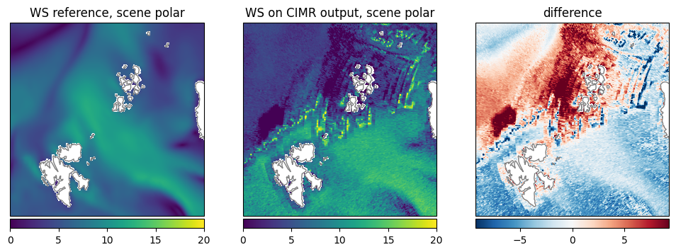
Fig. 22 Comparison of WS between reference dataset and retrieval.

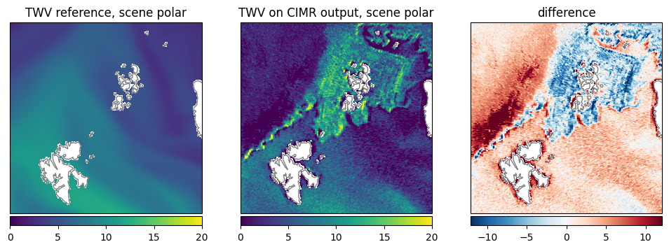
Fig. 23 Comparison of TWV between reference dataset and retrieval.

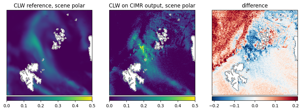
Fig. 24 Comparison of CLW between reference dataset and retrieval.

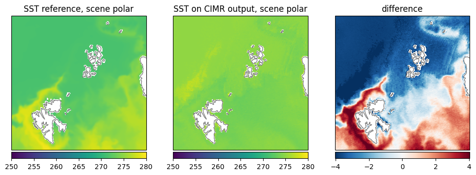
Fig. 25 Comparison of SST between reference dataset and retrieval.

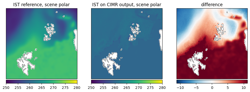
Fig. 26 Comparison of IST between reference dataset and retrieval.

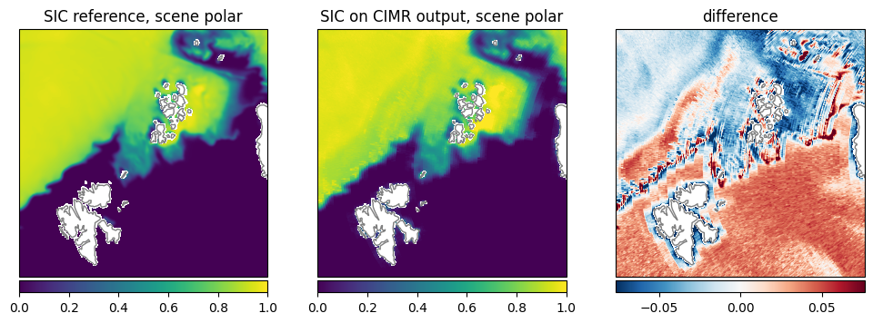
Fig. 27 Comparison of SIC between reference dataset and retrieval.

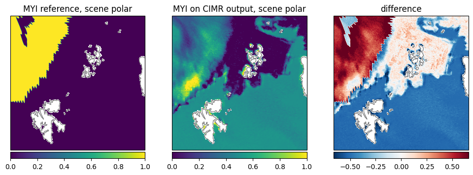
Fig. 28 Comparison of MYI between reference dataset and retrieval.

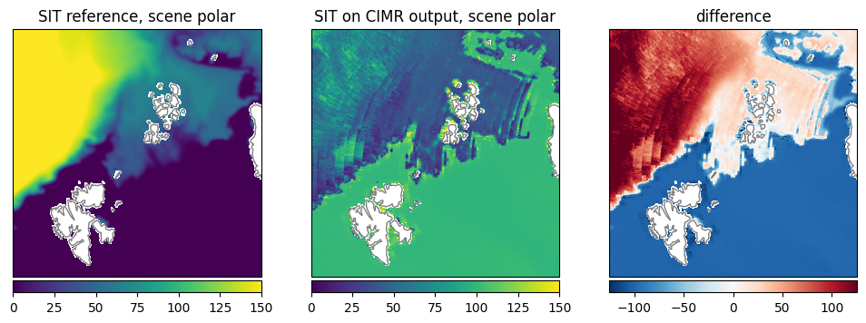
Fig. 29 Comparison of SIT between reference dataset and retrieval.

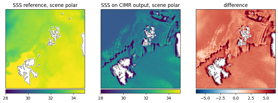
Fig. 30 Comparison of SSS between reference dataset and retrieval.

A summary of the performance of the retrieval on the L1b data compared to the reference dataset, i.e. mean difference (BIAS) and RMSD is shown in Table 6. For the different variables and observation directions. The results for the combined directions between the individual forward and backward scan results. The mean difference (BIAS) is very small for the SIC, CLW and MYI, while the other variables also show good performance. The standard deviation of the difference is a measure of how far the results spread around the mean difference. TWV and WS show very high values, but also the SSS and SIT values are quite large. The SIC as the value with the smallest bias, also has very low spread.

calculate_overall_performances([scenep], [gdata_true], ["forward","backward","combined"], [1]) |> x-> markdown_table(x,"multi parameter retrieval on the SCEPS polar scene. Forward (fw) and backward (bw) scans are shown separately and combined (cb).","polar-truth-combined") |> x->display("text/markdown",x) 

Table 6 Performance metric for multi parameter retrieval on the SCEPS polar scene. Forward (fw) and backward (bw) scans are shown separately and combined (cb).

Variable	fw mean(diff)	fw std(diff)	bw mean(diff)	bw std(diff)	cb mean(diff)	cb std(diff)
WS [m/s]	0.128	4.727	0.045	4.717	0.080	4.724
TWV [kg/m²]	-1.915	5.743	-2.031	5.781	-1.984	5.756
CLW [kg/m²]	-0.017	0.098	-0.016	0.097	-0.017	0.097
SST [K]	1.452	2.395	1.458	2.402	1.456	2.400
IST [K]	-5.467	6.178	-5.470	6.174	-5.469	6.176
SIC [1]	-0.001	0.054	-0.000	0.054	-0.001	0.052
MYI [1]	0.179	0.415	0.180	0.415	0.180	0.415
SIT [cm]	22.468	85.845	22.929	85.745	22.724	85.796
SSS [ppt]	-3.797	1.428	-3.819	1.452	-3.808	1.440

For a better insight into the different comparisons, namely, the retrieval on the simulator input and the reference data, we illustrate a comparison of the SIC for the forward and backward scan in Fig. 31. The comparison of the retrieval on the input data and the reference data shows a very small difference, as expected. The difference is only visible at the ice edges and at the intermediate ice concentration where slight scan pattern are visible from the simulated L1b data.

using Statistics
#DRAFT: plot reference, forward and backward with corresponding differences
#layout: 3x3, first row: reference, forward, difference to reference
#second row: retrieved on CIMR input, backward, difference to reference
#third row: difference bteween reference and retrieved, difference between forward and backward, empty

#reference is in variable gdata_true
#retrieved on CIMR input is in variable gdata
#retrieved on CIMR output is in variable data which is a Dict with keys "forward" and "backward"

#variable ranges

mmdict=Dict("ws"=>[0,20],"twv"=>[0,20],"clw"=>[0,0.5],"sst"=>[250,280],"ist"=>[250,280],"sic"=>[0,1],"myi"=>[0,1],"sit"=>[0,150],"sss"=>[25,40])

#variable names and units
labdict=Dict("ws"=>"wind speed [m/s]","twv"=>"total water vapor [kg/m²]","clw"=>"cloud liquid water [kg/m²]","sst"=>"sea surface temperature [K]","ist"=>"ice surface temperature [K]","sic"=>"sea ice concentration [1]","myi"=>"multi year ice fraction [1]","sit"=>"first year ice thickness [cm]","sss"=>"sea surface salinity [ppt]")

sic = getfield(gdata_true, :sic)

scene="polar"
#varname="twv"
for varname in ["sic"]#["ws","twv","clw","sst","ist","sic","myi","sit","sss"]

    #get variables from dicts for given varname
    reference = getfield(gdata_true,Symbol(varname))
    input_retrieved = getfield(gdatap,Symbol(varname))
    forward = getfield(data["forward"], Symbol(varname))
    backward = getfield(data["backward"], Symbol(varname))

    #calculate maximum min max for difference plot for comparison
    diffmax=max(quantile(filter(!isnan, abs.(forward - backward)[:]), 0.95),
    quantile(filter(!isnan, abs.(reference - backward)[:]), 0.95),
    quantile(filter(!isnan, abs.(reference - forward)[:]), 0.95),
    quantile(filter(!isnan, abs.(reference - input_retrieved)[:]), 0.95))

    #colorbar_orientation = "horizontal"
    colorbar_orientation = "vertical"

    mins, maxs = mmdict[varname]
    fig = pyplot.figure(figsize=(15, 13))
    #fig.suptitle(labdict[varname])

    # upper left: reference
    ax = fig.add_subplot(331, projection=ccrs)
    im = ax.imshow(reference, vmin=mins, vmax=maxs, extent=leaextent, transform=ccrs)
    ax.set_title("$(labdict[varname]) reference")
    pyplot.colorbar(im, orientation=colorbar_orientation, pad=0.01)

    # upper middle: forward
    ax = fig.add_subplot(332, projection=ccrs)
    ax.set_title("retrieved $varname on CIMR output, forward")
    im = ax.imshow(forward, zorder=1, extent=leaextent, vmin=mins, vmax=maxs)
    ax.coastlines(color="gray")
    pyplot.colorbar(im, orientation=colorbar_orientation, pad=0.01)

    # upper right: difference reference - forward
    ax = fig.add_subplot(333, projection=ccrs)
    ax.set_title("difference reference - forward")
    im = ax.imshow(reference - forward, vmin=-diffmax, vmax=diffmax, extent=leaextent, transform=ccrs, cmap="RdBu_r")
    pyplot.colorbar(im, orientation=colorbar_orientation, pad=0.01)

    # middle left: input_retrieved
    ax = fig.add_subplot(334, projection=ccrs)
    ax.set_title("retrieved $varname on CIMR input")
    input_retrieved[landmask].=NaN
    im = ax.imshow(input_retrieved, zorder=1, extent=leaextent, vmin=mins, vmax=maxs)
    ax.coastlines(color="gray")
    pyplot.colorbar(im, orientation=colorbar_orientation, pad=0.01)

    # middle middle: backward
    ax = fig.add_subplot(335, projection=ccrs)
    ax.set_title("retrieved $varname on CIMR output, backward")
    backward[landmask].=NaN
    im = ax.imshow(backward, zorder=1, extent=leaextent, vmin=mins, vmax=maxs)
    ax.coastlines(color="gray")
    pyplot.colorbar(im, orientation=colorbar_orientation, pad=0.01)

    # middle right: difference reference - backward
    ax = fig.add_subplot(336, projection=ccrs)
    ax.set_title("difference reference - backward")
    im = ax.imshow(reference - backward, vmin=-diffmax, vmax=diffmax, extent=leaextent, transform=ccrs, cmap="RdBu_r")
    ax.coastlines(color="gray")
    pyplot.colorbar(im, orientation=colorbar_orientation, pad=0.01)

    # lower left: difference reference - input_retrieved
    ax = fig.add_subplot(337, projection=ccrs)
    ax.set_title("difference reference - CIMR input retrieved")
    im = ax.imshow(reference - input_retrieved, vmin=-diffmax, vmax=diffmax, extent=leaextent, transform=ccrs, cmap="RdBu_r")
    ax.coastlines(color="gray")
    pyplot.colorbar(im, orientation=colorbar_orientation, pad=0.01)
    
    # lower middle: difference forward - backward
    ax = fig.add_subplot(338, projection=ccrs)
    ax.set_title("difference forward - backward")
    im = ax.imshow(forward - backward, vmin=-diffmax, vmax=diffmax, extent=leaextent, transform=ccrs, cmap="RdBu_r")
    ax.coastlines(color="gray")
    pyplot.colorbar(im, orientation=colorbar_orientation, pad=0.01)

    #done
    #add space between subplots
    pyplot.subplots_adjust(wspace=0.05, hspace=0.08)

    plot_with_caption(fig, "Comparison of $(labdict[varname]) between reference dataset and retrieval Uppper row: reference, forward, difference to reference. Middle row: retrieved on CIMR input, backward, difference to reference. Lower row: difference between reference and retrieved, difference between forward and backward, empty.", "ref_full_comparison_$(varname)")

end

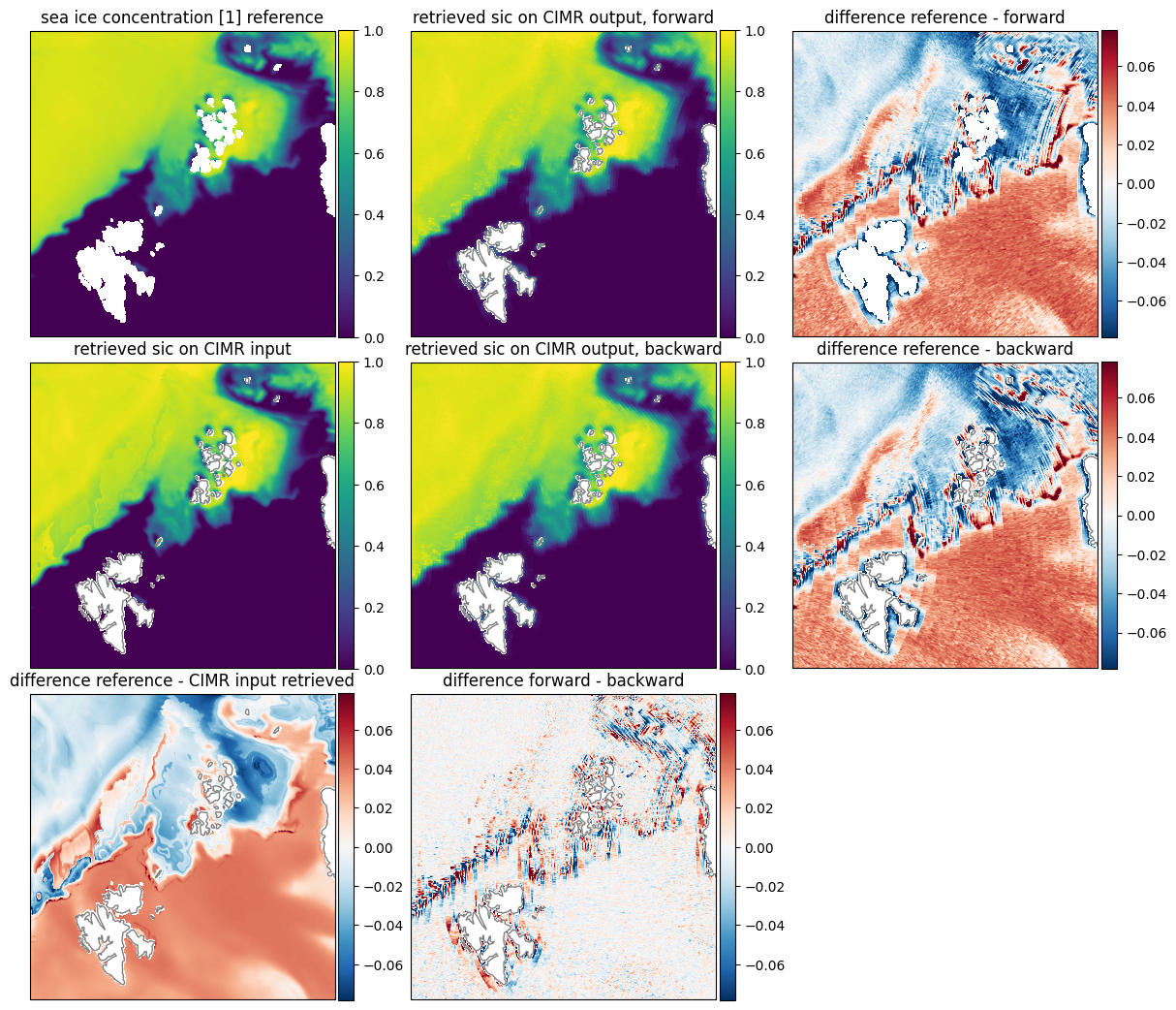
Fig. 31 Comparison of sea ice concentration [1] between reference dataset and retrieval Uppper row: reference, forward, difference to reference. Middle row: retrieved on CIMR input, backward, difference to reference. Lower row: difference between reference and retrieved, difference between forward and backward, empty.

Correction of OZA variation

The SCEPS polar scene in the simulated CIMR L1b format shows a strong variation with the individual scans due to slight variation in OZA. As a first attempt we correct this variation empirically as described in Correction for variation in incidence angle and apply the retrieval to the corrected data.

vmin=60
vmax=260
cmap = pyplot.cm.prism;
rows = ["v","v corrected","h","h corrected"]
let (fig,axs) = pyplot.subplots(4,4,figsize=[12,12])
    for (i,band) in enumerate(["C_BAND","X_BAND","KU_BAND","KA_BAND"])
        cbanddata=get_data_for_band(fns.scenep.l1b,band,"forward")
        cbanddata_corr=get_data_for_band(fns.scenep.l1b,band,"forward",oza_corr=true)
        lat, lon = cbanddata.lat, cbanddata.lon

        vproj=project_data_to_area_nn(cbanddata.v, lat, lon, lea)
        c=axs.flat[4*(i-1)+0].imshow(vproj,cmap=cmap,vmin=vmin,vmax=vmax)
        vproj=project_data_to_area_nn(cbanddata_corr.v, lat, lon, lea)
        c=axs.flat[4*(i-1)+1].imshow(vproj,cmap=cmap,vmin=vmin,vmax=vmax)
        vproj=project_data_to_area_nn(cbanddata.h, lat, lon, lea)
        c=axs.flat[4*(i-1)+2].imshow(vproj,cmap=cmap,vmin=vmin,vmax=vmax)
        vproj=project_data_to_area_nn(cbanddata_corr.h, lat, lon, lea)
        c=axs.flat[4*(i-1)+3].imshow(vproj,cmap=cmap,vmin=vmin,vmax=vmax)
        #pyplot.colorbar(c)
    end
    for i in 1:4
        fig.text(0.1, 0.82 - (i-1)*0.2, ["C","X","KU","KA"][i], va="center", ha="center", rotation="vertical", fontsize=16)
        fig.text(0.2 + (i-1)*0.2, 0.9,rows[i] , va="center", ha="center", fontsize=16)
    end
    for ax in axs.flat
        ax.axis("off")
    end
    #display("image/png",fig)
    plot_with_caption(fig, "Illustration of OZA correction for the forward scan for the four bands C, X, KU, KA. The first and third column shows the original data in v and h polarization, the second and fourth column the data after OZA correction in v and h polarization, respectively.", "oza_correction")
end

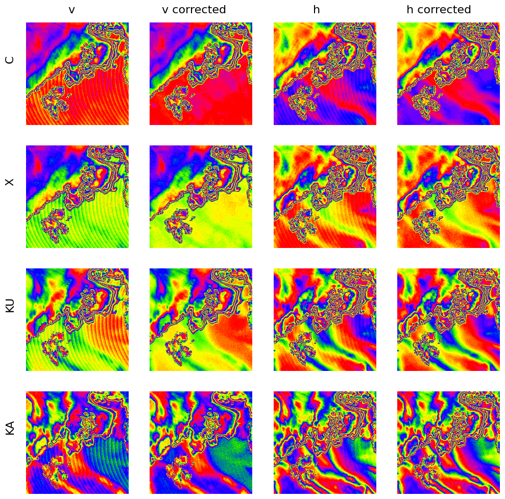
Fig. 32 Illustration of OZA correction for the forward scan for the four bands C, X, KU, KA. The first and third column shows the original data in v and h polarization, the second and fourth column the data after OZA correction in v and h polarization, respectively.

The color map shown in Fig. 32 is a cyclic color map, where small differences are visible as changes in color, while the color itself has no meaning in terms of the absolute value as it occurs multiple times for different values. This is useful to illustrate small differences in homogeneous areas at different absolute values. In this case, the repetitive pattern of the OZA can be seen in the data in the vertical and horizontal polarization, while this pattern is mostly removed in the corrected data. Only in KA-band at vertical polarization the OZA pattern is still slightly visible at the bottom right part of the image.

scenepnc = Dict()
for dir in ["forward","backward"]
    test2datac,test2derror,lat,lon=project_data(fns.scenep.l1b,"C_BAND",dir)
    x,y=lltoxy.(lat,lon) |> x-> (first.(x),last.(x))
    pygc.collect()
    GC.gc()
    dat,err,res=run_oem(deepcopy(test2datac))
    scenepnc[dir] = (; dat, err, res, x, y, lat, lon)
end

Here we show the retrieval applied on the backward scan of the uncorrected data Fig. 33 and corrected Fig. 34 data as comparison. The scan lines are mainly visible in variables where small changes in brightness temperatures have a big impact on the retrieval result. It is least visible over high ice concentrations and thus in the multi year ice fraction and also in the sea ice concentration retrieval in general.

let fig = plot_all_params(scenepnc,"backward",swath=false,mask=(:sic,:land),errors=:false)
    description = "The uncorrected data shows significant OZA variation in the retrieved quantities."
    return plot_with_caption(fig,description,"uncorrected_all_params")
end

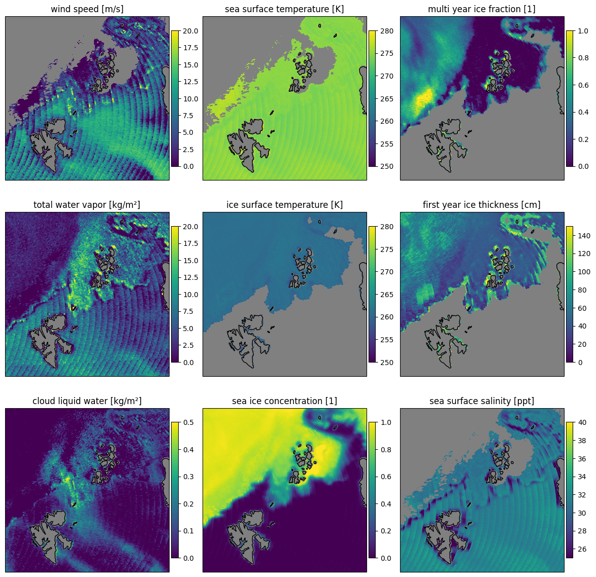
Fig. 33 The uncorrected data shows significant OZA variation in the retrieved quantities.

let fig= plot_all_params(scenep,"backward",swath=false,mask=(:sic,:land),errors=:false)
    description = "The backward scan of the corrected data has less OZA variation and more consistent retrieval results compared to the uncorrected data."
    return plot_with_caption(fig,description,"corrected_all_params")
end

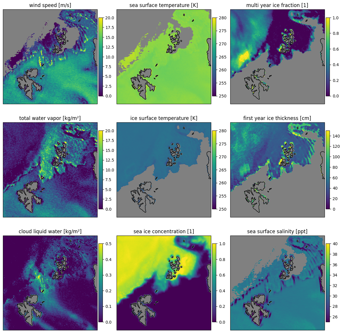
Fig. 34 The backward scan of the corrected data has less OZA variation and more consistent retrieval results compared to the uncorrected data.

Saving results (Example)

A few functions can be called to start the processing of CIMR L1b data and transform the result to a netCDF file. An example is shown here. We start with the project_data function to get to a common grid for all channels. On this we perform the retrieval using the run_oem function. The results are then stored in a named tuple with the with data, err and lat and lon keys for each viewing direction. This is stored for each viewing direction in another named tuple with the corresponding fields forward or backward. On this nested structure we can call the store_output function to save the results to a netCDF file.

# example to write out a file
#forward 
findata,finerror,flat,flon=project_data(fns.scene2.l1b,"C_BAND","forward")
fdat,ferr,fres,fit=run_oem(findata,band_error=finerror)
#backward
bindata,binerror,blat,blon=project_data(fns.scene2.l1b,"C_BAND","backward")
bdat,berr,bres,bit=run_oem(bindata,band_error=binerror)

thedata=(;forward=(;data=fdat,err=ferr,lat=flat,lon=flon,res=fres,it=fit),
         backward=(;data=bdat,err=berr,lat=blat,lon=blon,res=bres,it=bit))

store_output("test2_forward.nc",thedata,"ease2_nh");

(xsize, ysize, length(x), length(y)) = (1440, 1440, 1440, 1440)

sys:1: RuntimeWarning: invalid value encountered in cast

Summary

The Multi Parameter Retrieval MPR, has been demonstrated on the two CIMR DEVALGO test cards, as well as on the SCEPS polar scene. For the two DEVALGO test cards, the retrieval was applied on the input data to the CIMR simulator, as well as on the L1b data, which is the output of the CIMR simulator. This way of performance evaluation is used to assess the impact of the satellite characteristics on the retrieval, in particular the combination of different resolutions of the channels. As a performance metric for these scene, the mean difference is calculated, which can be referred to as BIAS. In addition the standard deviation of differences are assessed which is technically the mean difference from the BIAS. The performance of the retrieval on the L1b data is very similar to the performance on the input data. This is expected as the simulator is slightly modifying the input brightness temperatures. The differences are only visible at the ice edges and at the intermediate ice concentration where slight scan pattern are visible from the simulated L1b data. The performance of the retrieval on the SCEPS polar scene is also very similar to the performance on the DEVALGO test cards. The OZA variation in the SCEPS polar scene is corrected empirically and the retrieval is applied to the corrected data. The visible scan lines from the OZA variation are mainly removed in the all retrieved quantities on the OZA corrected data. The addition of the sea surface salinity to the retrieval could be accomplished but the sea surface salinity comes with a high uncertainty in this retrieval. Interestingly, the retrieved SSS is showing the OZA pattern, even though it is mostly influenced by L-band TBs which is most sensitive to salinity. At L-band CIMR only observes with one single feed horn so that OZA variation is not present for neighboring scan lines. The OZA pattern in the SSS retrieval is propagating from the strong OZA effect on wind speed, which can be seen in multiple frequencies, including KU-band and KA-band, where the OZA effect is strongest. In the OZA corrected version, no pattern is visible in the SSS retrieval. Additional work will need to be done to understand how this OZA pattern propagates through different frequencies and what it means for retrievals of other parameters such as wind speed or temperature.