Background and justification of selected algorithm

Introduction

Ocean salinity is a key physical-chemical variable that critically contributes to the density-driven global ocean circulation and the Earth’s climate [Siedler et al., 2001]. The Sea Surface Salinity (SSS) is affected by (and thus reflects) the air-sea freshwater fluxes (Wust [1936]; Schmitt [2008]; Durack et al. [2012]; Skliris et al. [2014]; Zika et al. [2015]), ice formation/melting, river runoff, horizontal advection and vertical exchanges through mixing and entrainment. It also provides fundamental information for ocean bio-geochemistry through its links with the carbonate system (Land et al. [2015];Fine et al. [2017]). Stable fresh surface salinity layers (such as river plumes, rain-induced lenses) on top of saltier and denser deep waters can inhibit the upper-ocean mixing generated by intense atmospheric events (e.g., wind bursts, tropical cyclones) due to so-called barrier layer effect (e.g., Lukas and Lindstrom [1991]; Balaguru et al. [2012]). This suggests that mixed layer salinity can actively impact air-sea interactions from local to synoptic scales. Given its importance for many key ocean and climate processes, the SSS has been recognized as an Essential Climate Variable (ECV) by the Global Climate Observing System (GCOS) program. [Bingham et al., 2002] examined the global distribution of historical (1874-1998) in situ SSS observations measured at 5 m or less in depth from the World Ocean Database 1998 (WOD98) and showed how poorly SSS was sampled by the end of the 1990s, despite a peak period of ocean sampling (including near surface salinity) during the World Ocean Circulation Experiment (WOCE, 1990-1998). The Global Ocean Data Assimilation Experiment (GODAE) group, therefore, estimated that it would be necessary to develop global SSS measurements from both in situ sensor networks and dedicated satellite missions to reach an accuracy of about 0.1-0.2 pss at monthly and 100 \(\times\) 100 km\(^2\), or 10-day and 200 \(\times\) 200 km\(^2\) scales. Tremendous efforts to reach this goal using in situ sensor networks have been carried out by the ocean science community since the early 2000s. At global scale, the large increase in salinity data sampling is dominantly associated with the invention and deployment of the Argo profiler network. Since reaching its full planned capacity in 2007, the network includes ~3000 Argo floats in the global Ocean providing at least one salinity cast every 10 days in a 3\(^{\circ}\times\)3\(^{\circ}\) cell (see Notarstefano [2022]).
In addition to Argo floats which profile to the top 2 km of the global ocean column, near surface salinity is monitored by thermosalinographs (TSG) on board numerous ships of opportunity and research vessels.
These TSGs are installed and maintained on board ships via international programs such as the Global Ocean Surface Underway Data (GOSUD; Alory et al. [2015]) and the Shipboard Automated Meteorological and Oceanographic System (SAMOS; Smith et al. [2009]), as well as a growing number of deployments of surface drifters equipped with salinity sensors.

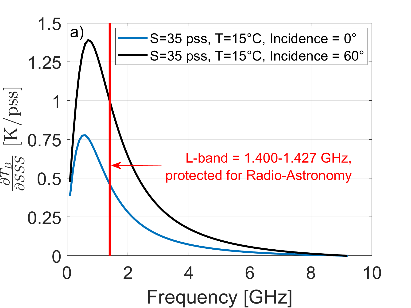
Fig. 1 Sensitivity of the ocean surface microwave brightness temperature to Salinity (First Stokes parameter) as a function of electromagnetic frequency and incidence angle (blue curve=0°, black curve=60°) and for a water body with salinity of 35 pss and temperature of 15°C.

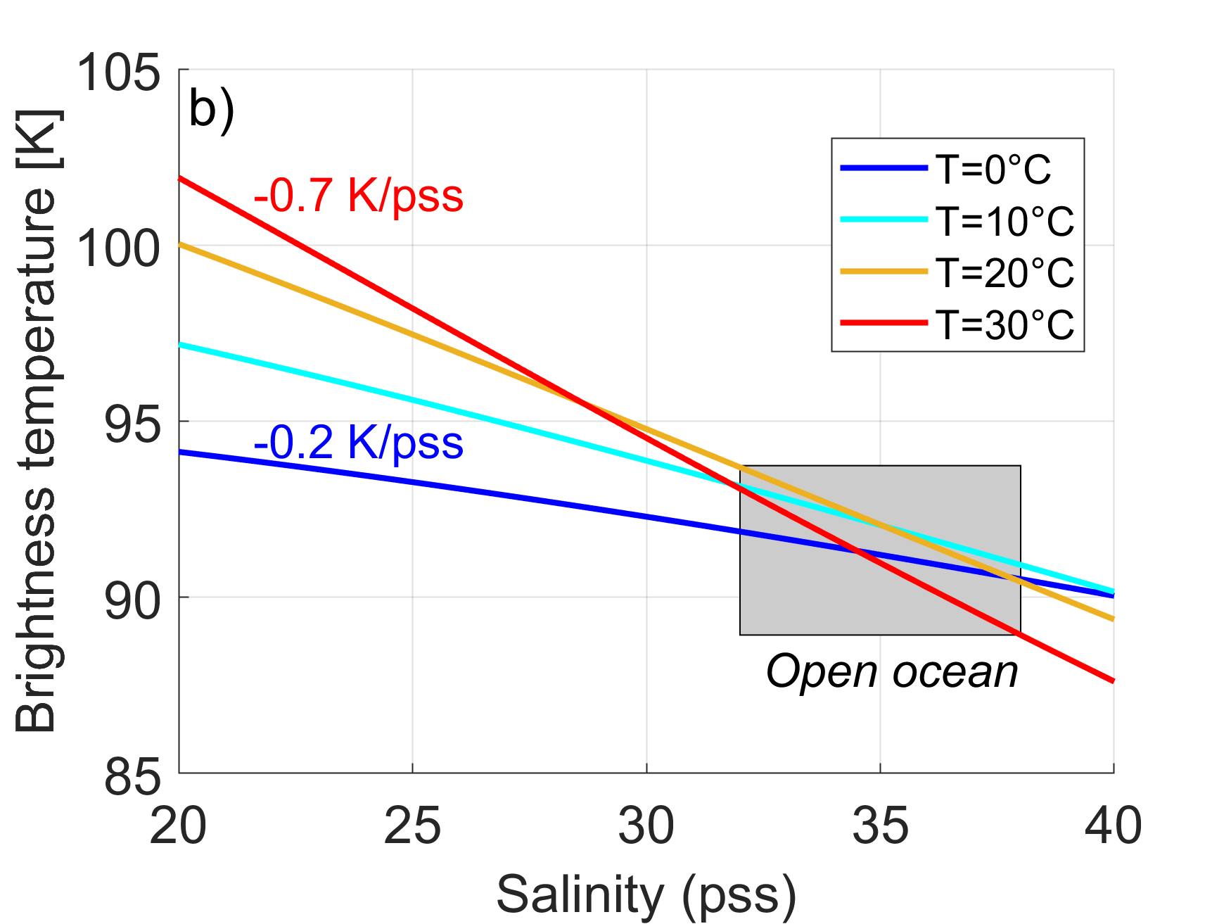
Fig. 2 First Stokes parameter of the Brightness temperature \((T_{esh}+T_{esv})/2\) changes at 1.4 GHz and nadir of the perfectly flat sea surface as a function of salinity (x-axis) and temperature (colors). The gray domain indicates the range of SSS values mostly encountered in the open ocean.

Despite its oceanographic importance, SSS is an ocean ECV that only started to be estimated from space about ten years ago with the launch of the Soil Moisture and Ocean Salinity (SMOS) mission by the European Space Agency (ESA) in November 2009. The SMOS mission was then followed by the NASA/CONAE Aquarius/SAC-D mission also focused on the sea surface salinity. Both missions had an overlapping period between June 2011 and mid-2015. Next came the NASA Soil Moisture Active-Passive (SMAP) mission launched in early 2015, which also monitors SSS. SMOS and SMAP operation periods overlapped with Aquarius only during about four months (February to June 2015). The primary sensors onboard these three missions are L-band microwave radiometers operating at ~1.4 GHz (wavelength=21cm). When accurate corrections for external contributions to the measured radiometer signal are applied (e.g., radiation from the Sun and celestial radio sources, reflection/emission due to sea surface roughness, and temperature), the SSS can be estimated from L-band brightness temperature TB (Font et al. [2004]; Lagerloef et al. [1995]). The feasibility of the measurement of SSS at L-band was demonstrated in the 1970s in a number of field campaigns from aircraft (Droppleman et al. [1970]), from a bridge which spans the Cape Cod canal (Swift [1974]), and even with a satellite radiometer from the short-lived (2-week) Skylab S-194 mission (Lerner and Hollinger [1977]). It took more than 40 years after the aforementioned pioneer experiments to develop and implement instruments to measure SSS regularly from space with sufficient accuracy and spatial resolution to address the GODAE recommendation. Two major technological factors limit L-band SSS measurements from space. First, at low microwave frequencies (decimeter wavelengths), classical radiometer sensors require large antenna size of ~3 to 8 m in diameter to meet a useful spatial resolution on the ground (100-150 km at most, 30-50 km wished for). Such large antenna technologies were not available before the late 1990s. Second, while being optimal in low microwave frequencies (see Fig. 1 and Fig. 2), the sensitivity of the sea surface brightness temperature to salinity at 1.4 GHz and vertical (VV) polarization varies only between (\(\partial T_{B}/\partial SSS\))~ -0.5 to -1 K/pss for incidence angles from 0° to 60° at characteristic ocean conditions (SSS= 35pss and Sea Surface Temperature (SST)=15°C). This sensitivity to SSS remains relatively small compared to (i) noise characteristics of available radiometers (~0.3 to 2 K) and (ii) the small range of natural variability of SSS in the open ocean (32 to 38 pss). Finally, as illustrated in Fig. 2, (\(\partial T_{B}/\partial SSS\)) also decreases with decreasing SST from ~-0.7 K/pss at 30°C to ~ -0.2 K/pss at 0°C making SSS estimation in the high latitude cold waters even more challenging than in the tropics. Given the sensitivity of \(T_B\) to salinity at 1.4 GHz, very low noise radiometers and/or a large number of \(T_B\) observations for a given ocean scene within short integration times (~a few seconds) are required for accurate SSS estimations. Therefore, salinity satellite mission objectives are generally expected to be reached for SSS products obtained after spatio-temporal averaging of in-swath instantaneous data.

Historical Heritage

In the late 1960s, Sirounian [1968] and Paris [1969] recognized that ocean surface microwave emission in the 1 to 3 GHz range had measurable sensitivity to changes in ocean SSS. The first airborne salinity measurements were demonstrated in 1970 by Droppleman et al. [1970]. Combining aircraft mounted 1.4 GHz microwave and 11 µm infrared radiometers, they were able to observe strong SSS gradients near the mouth of the Mississippi River, and thus demonstrate the feasibility of 1.4-GHz passive radiometers to detect sea water salinity gradients. Multi-frequency (L-, X- and K-bands) microwave radiometer observations conducted by Hollinger [1971] from a research tower located off the island of Bermuda revealed the potential effect of sea surface roughness on L-band TB for wind speed conditions varying from calm to 15 m/s. Thomann [1976] used a system similar to Droppleman et al. [1970] to map ocean surface salinity in the Gulf of Mexico. As reviewed in Goodberlet et al. [1997], these early instruments could achieve an acceptable measurement accuracy only by averaging over time periods from 12 to 16 seconds. The averaging time was later reduced below 1 second using a NASA Langley built precise radiometer system (Blume et al. [1978]; Blume and Kendall [1982]) operating at 1.4 GHz (L-band) and 2.65 GHz (S-band). Its improved noise characteristics (and lower integration times) allowed improvement in spatial resolution and measurements in the Chesapeake Bay SSS that resolved ~0.5 km spatial scales. The dual-frequency radiometer system was also successfully operated from an aircraft (Kendall and Blanton [1981]) to measure quasi-synoptic salinity changes induced by the Savannah River plume along the coast of Georgia. A key model component for the salinity retrieval algorithm from microwave radiometer data is the model for the sea water dielectric constant, \(\epsilon_{sw}\). The semi-empirical Debye model was first proposed by Stogryn [1971] and re-analyzed by Klein and Swift [1977] to include new S-band and L-band data from the NASA 2-band radiometer. Shutko et al. [1982] further examined and refined the dependencies of ϵ on electromagnetic frequency, water temperature, and salinity. In addition, near nadir L-band measurements from the Bering Sea aircraft experiments as reported by Webster Jr et al. [1976] allowed for better characterization of wind speed dependence of the surface emissivity.

First attempts to measure SSS from space took place in 1968 aboard the Soviet Cosmos 243 and in 1973 aboard the Skylab S-194 satellite missions (Lerner and Hollinger [1977]). They utilized nadir looking L-band horizontal (HH) microwave radiometers with 3dB beam width of 15° corresponding to ~110 km ground footprint. Unfortunately, only a very limited amount of L-band radiometer data were collected and there were no in situ measurements available to validate SSS retrievals estimated from the satellite data. Nevertheless, the retrieved SSS was found correlating with climatological in situ salinity. Overall, these experiments showed that open sea SSS (i.e., away from the land and coasts) could be measured with an accuracy of ~2 pss, a promising early result. Based on these first aircraft and satellite experiments, Swift and McIntosh [1983] suggested a revised satellite concept to achieve an ideal precision of about 0.25 pss with a footprint spatial resolution of ~100 km. However, at that time, space agencies were primarily devoting efforts to develop missions to measure surface temperature (Advanced Very High Resolution Radiometers (AVHRRs) and Along-Track Scanning Radiometers (ATSRs)), surface dynamic topography (Geosat (GEOdetic SATellite)), wind stress (SEASAT A Scatterometer (SASS)), ocean color (Coastal Zone Color Scanner (CZCS)), and sea ice (scanning multichannel microwave radiometer (SMMR)). Mainly because of the technological challenges associated with the launch of sensors with large antenna size and the need for high radiometric sensitivity, salinity remote sensing was considered too costly and not given a high priority in the early 1980s. Interest in salinity remote sensing was renewed in the late 1980s with the development of an airborne demonstration instrument called the Electrically Scanning Thinned Array Radiometer (ESTAR), which was operated at 1.4 GHz and used the concept of aperture synthesis (Le Vine et al. [1990]) allowing an increase in cross-track spatial resolution. Small salinity variations typical of the open ocean were retrieved from the data acquired by the ESTAR interferometer during flights across a coastal current in Delaware and the Gulf Stream (Le Vine et al. [1998]). Such a system demonstrated that it was feasible to achieve high spatial and radiometric resolution at a reasonable cost for a potential 1.4 GHz satellite radiometer design. By the mid-1990s, the Scanning Low Frequency Microwave Radiometer (SLFMR) was built (Goodberlet and Swift [1993]) based on the similar concept as the ESTAR but with an improved radiometric resolution and adapted for light aircraft. Salinity in coastal and estuarine waters on the U.S. Atlantic coasts, as well as in the Australian Great Barrier reef waters have been mapped successfully using the SLFMR data acquired during several airborne campaigns (Robinson [1985]; Le Vine et al. [1998]; Miller et al. [1998]; Burrage et al. [2003]; Miller* and Goodberlet [2004]; Perez et al. [2006]).

A detailed review of remote sensing of SSS in coastal waters is provided in Klemas [2011]. A Passive-Active L-band System (PALS) (Wilson et al. [2003]) providing coincident scatterometer and radiometer airborne L-band data was developed to better characterize the sea surface roughness impact on L-band TB. This instrument was deployed on ocean flights across the Gulf Stream in an attempt to illustrate the use of active scatterometer data to correct the impact of surface roughness on passive radiometer data (Yueh et al. [2001]). The PALS design and data provided the basis for the NASA Aquarius and SMAP instrument designs. In 1995, during the “Soil Moisture and Ocean Salinity” Workshop organized at the ESA ESTEC (European Space Research and Technology Centre, Noordwijk, the Netherlands), possible techniques to remotely measure SSS from space were discussed. The two most suitable approaches were identified to be L-band microwave radiometry using either real or synthetic, aperture antenna design. The use of a real aperture antenna with moderate size (diameter < 3m) eases sensor integration into a launch vehicle and better fulfills satellite weight constraints but results in lower spatial resolution on the ground. This option was realized for the Aquarius mission with a moderately large antenna (reflector diameter ~2.5m) used in the push broom mode. Another concept was realized for the SMAP mission, which has a relatively large deployable mesh antenna reflector of 6 meters in diameter. Both Aquarius and SMAP instruments were designed with combined active and passive measurements. The second approach involves the use of interferometric radiometers with a synthetic aperture antenna allowing TB measurements at higher spatial resolution than with a real-aperture antenna of the same size. The ESTAR interferometric 1-D imaging concept evolved into a 2-D imager in the mid-1990s (Goutoule et al. [1996]). Its airborne prototype was made and operated (Bayle et al. [2002]) and then further evolved into the Microwave Imaging Radiometer with Aperture Synthesis (MIRAS), the instrument carried by the SMOS mission.

Justification of selected algorithm

The new satellite SSS era started with the Soil Moisture and Ocean Salinity (SMOS) mission, launched in 2009 under the auspices of the European Spatial Agency (ESA), the French Centre National d’Etudes Spatiales (CNES), and the Spanish Centre for the Development of Industrial Technology (CDTI). Followed by the National Aeronautics and Space Administration (NASA) Aquarius instrument from mid-2011 to mid-2015, it is today complemented by the NASA Soil Moisture Active-Passive (SMAP) mission. Initially dedicated to Soil Moisture measurements only, SMAP applications have been extended to include the SSS, which is available since early 2015. All instruments on-board these different missions follow an early 1970s historical heritage that demonstrated how passive microwave radiometer observations in the L-band (frequency~1.4 GHz, wavelength~21 cm) could be used to retrieve SSS. Tthe SSS measurement principle was successfully developed and demonstrated in the 1970s from various platforms (land-based bridge, aircrafts, towers, short-lived satellites, etc). The long delay until the final development and launch of the first satellite salinity sensor was mainly dictated by technological challenges associated with space delivery and deployment of large antennas. Indeed, to achieve a proper pixel resolution, a very large size (~3-8 m) radiometer antenna is needed for 1.4 GHz operations even from low polar orbits. There are major technological differences but also similarities between the three first satellite salinity missions. SMOS and SMAP spatial resolution (~40 km) is a factor 2-3 higher than Aquarius spatial resolution (~100 km - 150 km). Moreover, with their large swaths, observations cover almost the full globe in 3 days, while 7 days were needed in the case of Aquarius. Yet, Aquarius radiometric noise was significantly lower than SMOS or SMAP radiometric noise. For SMOS, image reconstruction errors are sources of specific and variable noise in the TB images (e.g., sun and land image aliasing in ocean scenes, noise floor errors …) and impact the quality of retrieved SSS from this sensor. But SMOS multi-angular viewing capability also provides a way to mitigate the noise in individual samples, thanks to a large number of TB acquisition for a given ocean target pixel. The Aquarius antenna emissivity was negligibly small, while the SMAP mesh reflector has an emissivity of about 0.2%, which needs to be accounted for in salinity retrieval. Moreover, the simultaneous acquisition of scatterometer and radiometer observations by Aquarius significantly helped to improve the correction for sea surface roughness effect. For SMOS and SMAP, retrieval algorithms must rely on external surface wind vector data, not always of sufficiently high quality to well characterize the actual impact of roughness on L-band passive sensors. For CIMR the case is different as higher frequency chanels can provide quasi-simulatneous SST and wind data.

Model for the dielectric constant of the seawater at L-band

The relative permittivity (also called dielectric constant) of the seawater, \(ε_{sw}(f, S, T)\), is a complex function dependent on \(f\), the electromagnetic frequency, as well as, temperature \(T\), and, salinity \(S\). It is a key component of the radiative transfer forward model used for sea surface salinity retrieval from L-band radiometer data, as the accuracy of SSS retrievals strongly depends on how well the dielectric constant is known as a function of these two geophysical parameters (Lang et al. [2016]). Models for \(ε_{sw}(f, S, T)\) at frequency \(f\)=1.4 GHz are still uncertain, particularly at low \((\le 8^{\circ}C)\) and high \((\ge 28^{\circ}C)\) SST. \(ε_{sw}(f, S, T)\) can be estimated at any frequency \(f\) within the microwave band from the Debye [1929] expression involving \(ε_{\infty}\), the electrical permittivity at very high frequencies, \(ε_{s}\) the static dielectric constant, \(\tau\) the relaxation time, \(\sigma\) the ionic conductivity, and \(ε_0\) the permittivity of free space, where \(ε_{s}\), \(\tau\) and \(\sigma\) are functions of temperature \(\it{T}\) and salinity \(\it{S}\). At the time the first salinity mission was developed, these functions had been evaluated historically by Stogryn [1971], Stogryn et al. [1995], Klein and Swift [1977], and Ellison et al. [1998]. Klein and Swift [1977] (denoted KS hereafter) modified the Stogryn [1971] model by using a different expression for the static dielectric constant \(ε_{s}(S,T)\), based on Ho and Hall [1973] and Ho et al. [1974] measurements at 2.6 and 1.4 GHz, respectively. The KS and Stogryn \(ε_{sw}\) models are valid for frequencies ranging from L- to X-bands (Meissner and Wentz [2004]; Meissner and Wentz [2012];Meissner et al. [2014]). Following SMOS pre-launch comparisons and analyses (Camps et al. [2004]; Wilson et al. [2004], Blanch and Aguasca [2004]), the KS model was selected in the Level 2 Ocean Salinity (OS) processor for the SMOS mission in the first phases post-launch (Team and others [2016]).
An alternative model function developed by Meissner and Wentz [2004] (denoted MW hereafter) fits the dielectric constant data to a double Debye relaxation polynomial that performs best at higher frequencies. The seawater dielectric data were obtained by inverting \(T_B\) measurements from the Special Sensor Microwave Imager (SSM/I) at frequencies higher than 19 GHz; measurements from Ho et al. [1974] were used to derive the model at the lower frequencies. The MW model function was recently updated by providing small adjustments to the Debye parameters based on including results for the C-band and X-band channels of WindSat and AMSR (Meissner and Wentz [2012];Meissner et al. [2014]). The MW model is used in the Aquarius and SMAP SSS retrieval algorithms (Meissner et al. [2018]). Dinnat et al. [2014] analyzed the difference in SSS retrieved by SMOS and Aquarius radiometers and found that both instruments observe similar large scale patterns, but also reported significant regional discrepancies (mostly between +/- 1 pss). SMOS SSS was found generally fresher than Aquarius SSS (within 0.2-0.5 pss depending on latitude and SST), except at the very high southern latitudes near the ice edge and in a few local (mostly coastal) areas. It was found that the differences exhibit large-scale patterns similar to SST variations. To investigate its source, Dinnat et al. [2014] reprocessed the Aquarius SSS, including the calibration, using the KS \(ε_{sw}\) model that is used in SMOS processing. This reprocessing decreases the difference between Aquarius and SMOS SSS by a few tenths of a pss for SST between 6°C and 18°C while warmer waters show little change in the difference. Water colder than 3°C shows mixed results, probably due to a complex mix of error sources, such as the presence of sea ice and rough seas. The comparison of the reprocessed Aquarius SSS with in situ data from Argo shows an improvement of a few tenths of a pss for temperatures between 6°C and 18°C. In warmer waters, both the nominal and reprocessed Aquarius data, as well as SMOS data, have a fresh SSS bias. For very cold waters (less than 3°C), the reprocessed Aquarius data using the KS model show significant degradation of the SSS in comparison with the Argo, in turn suggesting that the KS model might be in error in the lowest sea surface temperature regime. Direct laboratory measurements of the \(ε_{sw}\) at 1.413 GHz and SSS=30, 33, 35, and 38 (Lang et al. [2016]) were used to develop a new model (Zhou et al. [2017]) by fitting the measurements with a third-order polynomial. This new L-band \(ε_{sw}\) model has been compared with KS and MW. The authors claimed that this new model function gives more accurate SSS at high (25°C to 30°C) and low (0.5°C to 7°C) SSTs than other existing model functions. Laboratory measurements at low SSS lead to a small increase in the accuracy of the model function. Although the model showed improvements in salinity retrieval, it had an inconsistent behavior between partitioned salinities. To overcomme these problems, two new parametrizations were recently developed based on one hand on SMOS satellite multi-angular brightness temperature measurements by Boutin et al. [2021] (BV), and on the other hand on new George Washington laboratory measurements by Zhou et al. [2021] (hereafter denoted GW2020). These two approaches are fully independent. The brightness temperatures Tb simulated through the BV and GW2020 parametrizations agree particularly well for most SSS and SST conditions commonly observed over the open ocean, and better than with earlier parametrizations previously used in the SMOS, SMAP and Aquarius SSS retrievals. Nevertheless, uncertainty remains below 10°C where a ~0.1K relative difference between the two models is observed.

Recently, Le Vine et al. [2022] compared available models in the context of how well they represent the dielectric constant of sea water at 1.4 GHz. Among the criteria applied were the recent measurements at the George Washington University of the dielectric constant at 1.4 GHz. As reviewed, in the two models, BV and MW, parameters were tuned to optimize the science retrieval algorithm by choosing the model parameters to minimize the differences between radiative transfer simulations of the brightness temperature and the TB actually observed by the satellite. These two models are close to the measurements but diverge in some significant respects. This is particularly evident in the temperature dependence of the real part. The BV model was tuned to optimize the retrieval of salinity from SMOS observations of brightness temperature at 1.4 GHz. The tuning was done on the temperature dependence of the static term, which is strongly coupled to the real part. The MW model is a double Debye resonance model intended to cover a large range of higher frequencies and the tuning was done to fit the satellite observations from Windsat and SSM/I in this higher range and particularly near 37 GHz.

Three of the models have been used in remote sensing of salinity: KS and BV have been used in SMOS retrievals and MW was used for Aquarius and is now used for retrieving salinity from soil moisture active passive (SMAP). In addition, a combination of the MW and KS model has been used in the combined active passive (CAP) algorithm for retrievals from Aquarius and SMAP. While these models have been used quite successfully to retrieve salinity, this success does not guarantee that they are a good representation of the dielectric constant of sea water. For salinity typical of the open ocean, 32<S<38 psu, the differences in the dependence of the models on S are on the order 0.1 K, which is acceptable. As found by Le Vine et al. [2022], except for cold temperatures, KS appears to be a better fit to the dielectric constant at 1.4 GHz. Because BV and MW are satellite sensor-dependent and tuned to best fit their specific datasets, and because KS seems biased in low SSTs, as a first step, we plan here to rely on the GW2020 empirical model based the most recent George Washington laboratory measurements as describe in Zhou et al. [2021].

Model for correcting the sea surface roughness emission

The current status in the development of forward models to estimate and correct for the sea surface roughness contribution to L-band TB measured at antenna level can be summarized as follows. To first order, Geophysical Model Functions (GMF) developed are dependent on the surface wind speed. There is a good agreement between L-band GMFs used in the latest versions of Aquarius, SMAP, and SMOS products (V5 for Aquarius, RSS V5 for SMAP, JPL V4 for SMAP and ESA V772 for SMOS) (Yin et al. [2016]; Meissner et al. [2018]). The JPL CAP algorithm developped for Aquarius data (Yueh et al. [2014],Fore et al. [2016]) relies on a purely-empirical GMF for the roughness correction. In all other operational algorithms, a semi-empirical two-scale scattering model approach is used for that correction, such as in [Yin et al., 2016] for SMOS, and in [Meissner et al., 2018] for SMAP and Aquarius. Development and analysis of the two-scale model for ocean waves and resulting microwave ocean emissivities were presented in (Yueh [1997]) and (Yueh et al. [1994], Yueh et al. [1999]; Johnson [2006]; Ma et al. [2021]; Lee and Gasiewski [2022]), within which were published two-scale model algorithms that have been successfully used to date for the prediction of ocean wave influences on surface emission. Ocean foam (i.e., white capping) is an air–sea mixture caused by ocean wave breaking and is an additional surface process that strongly increases ocean surface emissivity (Monahan and O'Muircheartaigh [1986]; Stogryn [1972]; Reul and Chapron [2003]; Camps et al. [2005]) at microwave frequencies due to its near-blackbody behavior. As wind speed increases, ocean foam coverage also increases, resulting in a large discrepancy between two-scale emissivity calculations made with and without consideration of foam coverage. The quasi-blackbody models used for both foam emissivity and coverage are in themselves of limited accuracy due to the paucity of in situ observations for both foam coverage and emissivity that have been able to be made in conjunction with brightness temperatures from passive microwave instruments. In spite of numerous efforts to derive a suitable empirical relationship between foam coverage and ocean surface wind speed (Monahan and O'Muircheartaigh [1986]; Erickson et al. [1986]; Asher et al. [2002]; Bondur and Sharkov [1982]; Anguelova and Webster [2006]; Callaghan et al. [2008]), there is to date no universally accepted relationship between them due to the variable conditions under which foam is produced, as well as its spatial inhomogeneity. This shortcoming is especially true for breaking waves caused by shoaling. Smith et al. [2008] found that the differences in surface-referenced microwave brightness temperatures between WindSat observations and a two-scale model developed by Johnson [2006] were significant, especially in the zeroth-azimuthal-harmonic components of ocean brightness at a wind speed of 8–20 m/s. The discrepancy was largely due to foam coverage and emissivity models. They concluded that an empirical tuning process using observed satellite data is needed to model ocean surface emissivity with enough precision for general retrieval and data assimilation applications.

The limitations on the various purely physical published models on the ocean surface emissivity include a limited range of validity in frequency and incidence angle. Combined physical and empirical models have been used to correct for these shortcomings but do not necessarily permit extension of the models to arbitrary frequencies and incidence angles, as required for the design and development of new observation systems.

In this algorithm for CIMR, a full Stokes vector model for ocean surface emissivity based on the two-scale approach is used, applicable at arbitrary microwave frequencies, incidence and azimuth angles, and polarizations, and subsequently tuned at L-band within a limited set of selected model parameters against SMOS, Aquarius, and SMAP observations from 0- to 20-m/s wind speeds.

In the case of Aquarius, the direct use of scatterometer measurements significantly improves the accuracy of the surface roughness correction. While there is a consensus on the first-order wind-speed dependencies of the GMFs, the wind direction signature, the wave impact (significant wave height, wave-age), and the air/sea temperature dependencies of this correction still exhibit significant differences. Remaining uncertainties for these second order effects are still the subject of on-going research efforts.

Model for other geophysical contributions

In the SSS retrieval algorithm, accurate corrections associated with ionospheric, atmospheric, solar, and sky radiation contributions to the antenna measured brightness are needed.

The ionospheric correction commonly involve the use of the ratio of the third Stokes (U) parameter to the difference between the vertical and horizontal polarization channels (Yueh [2000],Le Vine and Abraham [2002],Vergely et al. [2014]). This helps to infer the rotation angle (geometry plus Faraday) across the ionosphere. Again, accurate calibration of the third Stokes parameter is still challenging. The ionospheric rotation estimates also rely on the first guess data, including the Total Electronic Content (TEC) and geomagnetic field data (Vergely et al. [2014]) for which uncertainties still remain.

For L-band, sources of atmospheric attenuation are due to absorption by oxygen, water vapor, and liquid water. The contribution from the atmosphere is found to be a few Kelvins on average, rather stable in space and time, with the dominant source of signal associated with oxygen. As presently implemented, atmospheric corrections used in salinity retrieval algorithms all rely on time interpolated and integrated vertical profiles of atmospheric pressure, temperature, relative humidity, and cloud water mixing ratio obtained from numerical weather forecast models (ECMWF or NCEP). The overall error in salinity retrievals due to the atmosphere is estimated to be less than 0.2 pss (e.g., Meissner et al. [2018]).

Correcting for the Sun and Sky direct and reflected radiation further demands accurate characterization of the antenna patterns, and sun, and sky TB at the time of acquisition. Models for the bi-static scattering coefficients of the sea surface at L-band are then also needed. Sun flux measurements made by he United States Air Force Radio Solar Telescope Network are used but remain uncertain to within 10%, which is significant for salinity retrieval algorithms as the Sun is an extremely bright source at 1.4 GHz (~\(10^6\) K). Bi-static sea surface scattering coefficient models are generally estimated using the Physical Optics (Reul et al. [2007]), or the Geometric Optics approaches (Khazâal et al. [2016],Meissner et al. [2018]). A practical rule for L-band measurements is to consider a reduced, by about 50 %, surface slope variance as a function of wind speed, as compared to optical data. Applied corrections remove the reflected galactic radiation correctly to about 90% as estimated in the Aquarius and SMAP cases (e.g., Meissner et al. [2018]). Remaining uncertainties from the rough ocean surface scattering models in the L-band, the TB map of the celestial sky, and the antenna gain pattern appear as sources of remaining ascending-descending biases in all the satellite data. Empirical corrections to best mitigate these remaining signals are currently under investigation. They are based on either alternative antenna gain-weighted sky maps obtained from the satellite data or rely on the multiple view capabilities of the instrument (e.g., use of the fore and aft-look for SMAP). Antenna gain-weighted sky maps can be derived from the acumulated radiometer direct observation of the sky as recorded during the regular cold-sky calibration maneuvers.

Being significantly warmer than the ocean water at L-band, land surfaces can significantly impact the ocean TB measured, and this over a 400 to 1000 km-wide band off the coasts of the major land masses. A correction for land entering the antenna side-lobes when the sensor observation gets close to the land has been derived from simulated TB (Meissner et al. [2018]). Such empirical corrections appear to be efficient globally to reduce the land-contamination biases in satellite SSS. Yet, uncertainties remain in the antenna gain patterns and the reference geophysical fields (e.g. coastal SSS, land TBs), which are used to model the expected ocean-land transition signal. Alternatively, corrections can also be successfully applied after the SSS has been retrieved from the uncorrected TB. These corrections, based on filtering largely biased estimates, are empirical adjustments, or based on advanced filtering of the salinity products (e.g., Boutin et al. [2018], Olmedo et al. [2017], Olmedo et al. [2018]). Accordingly, while the absolute salinity retrievals can degrade quickly as the footprint approaches land, the SSS Anomalies (SSSA) derived from satellites generally show coherent and informative signatures in many coastal zones (Boutin et al. [2018]; Grodsky et al. [2018]; Grodsky et al. [2019]).