Baseline Algorithm Definition

In the following sections, the Level-2 sea-ice concentration algorithm is further described. It consists in those steps:

The CIMR Level-2 SIC algorithm has 3 main steps (Fig. 3):

1. L1B remapping

2. Computation of intermediate SICs

3. Pansharpening for Level-2 SICs.

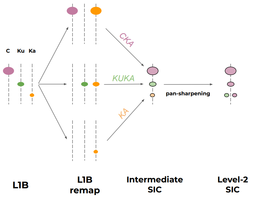
Fig. 3 Concept of the CIMR Level-2 SIC processing moving from input L1B TB (left) to Level-2 SICs (right). Ellipses and colours represent different microwave channels and their spatial resolution.

The first two steps above are applied three times, for three combinations of CIMR TB channels CKA, KUKA, and KA. CKA and KUKA combinations have both been tested in the EUMETSAT OSI SAF and ESA CCI Sea Ice projects [Lavergne et al., 2019]. The KU combination is the basis for the ‘Polarization Mode’ of the Bootstrap SIC algorithm [Comiso, 1986, Ivanova et al., 2015].

Table 4 introduces the three channel combinations used to prepare intermediate SICs in the Level-2 algorithm. The channel combinations are applied at different spatial resolutions, dictated by the lowest frequency of the set. They result in different accuracies (algorithms using C-band have better accuracy than those using only Ku and Ka channels). Note that the ‘<= X km’ in column ‘Resolution’ corresponds to the spatial resolution after the L1B remapping step and is thus at least the native resolution of the coarsest channel, but can also be better in case Backus-Gilbert techniques are implemented to take advantage of the overlap of FoVs (most relevant at C-band and away from the swath center at Ku-band).

Table 4 The three combinations of microwave channels used for the intermediate SICs.

Id	Channels	Resolution	Accuracy
CKA	\(\vec{T}=(\textrm{C-Vpol, Ka-Vpol, Ka-Hpol})\)	C (<= 15 km)	Excellent
KUKA	\(\vec{T}=(\textrm{Ku-Vpol, Ka-Vpol, Ka-Hpol})\)	Ku (<= 5 km)	Good
KA	\(\vec{T}=(\textrm{Ka-Vpol, Ka-Hpol})\)	Ka (4-5 km)	Poor

In Table 4, \(\vec{T}\) is the vector of brightness temperature input to the SIC algorithm. As described later, the definition of the SIC algorithms is slightly different for 2-dimensional algorithms (like KA: 2 imagery channels in \(\vec{T}\)) than for 3-dimensional algorithms (like CKA and KUKA: 3 imagery channels in \(\vec{T}\)).

The third step deploys a pan-sharpening methodology to combine pairs of intermediate SICs into the final Level-2 SICs. Pan-sharpening (aka image fusion, resolution enhancement, etc…) is a robust and straightforward method to improve the spatial resolution of a ‘base’ image by means of a ‘sharpener’ image. Pan-sharpening has been used in many fields of Earth Observation, mostly with higher-resolution optical imagery [Meng et al., 2019, Dadrass Javan et al., 2021]. In the context of passive microwave SIC it has been used in the NORSEX algorithm [Kloster, 1996] and more recently by Kilic et al. [2020] and in the context of the ESA CCI+ Sea Ice project.

In our case, the ‘base’ image can be the high-accuracy / coarse-resolution intermediate SIC from CKA and the ‘sharpener’ image can be the low-accuracy / fine-resolution intermediate SIC from KA. But other pan-sharpening combinations are possible. All pan-sharpened SICs should be made available in the Level-2 product (with one of them given prominent visibility as an entry point).

Table 5 Level-2 SICs, most of them obtained from pan-sharpening of intermediate SICs.

Id	Base image \(C_{LR}\)	Sharpener \(C_{HR}\)	Target Resolution	Target Accuracy
CKA	SIC from CKA	n/a	C (<= 15 km)	Excellent
CKA@KU	SIC from CKA	SIC from KUKA	Ku (<= 5 km)	Excellent
CKA@KA	SIC from CKA	SIC from KA	Ka (4-5 km)	Excellent
KUKA@KA	SIC from KUKA	SIC from KA	Ka (4-5 km)	Good

Table 5 lists candidate Level-2 SICs from CIMR, most of them obtained from pan-sharpening of intermediate SICs (CKA is directly from the intermediate SICs, without pan-sharpening). It is expected that one of these candidate Level-2 SICs will emerge as the best for most users and be flagged as the main L2 SIC product (e.g. CKA@KA).

Retrieval Method

As introduced above, the CIMR Level-2 SIC processing implements a series of steps that are run on three different combinations of microwave channels. Here we present the steps on a generic channel combination. We refer to this generic description later in the chapter when describing the actual implementation.

A generic formulation for a SIC algorithm and its uncertainties

At any microwave channel \(i\), and neglecting the contribution of the atmosphere to the signal, the TB recorded by CIMR over polar ocean areas is a linear combination of the typical signature of open water \(<T_{i}^{W}>\) (the open water tie-point), and of the typical signature of consolidated ice (100% SIC) \(<T_{i}^{I}>\) (the sea ice tie-point). The weighting between the two signatures is the SIC (noted \(C\)). Considering \(n\) microwave channels leads to:

(1)\[\begin{split} \left \{ \begin{array}{c} T_{1} = (1 - C) \times <T_{1}^{W}> + C \times <T_{1}^{I}> \\ ... \\ T_{n} = (1 - C) \times <T_{n}^{W}> + C \times <T_{n}^{I}> \end{array} \right. \end{split}\]

where \(<T>\) stands for the average \(T\).

By re-arranging the terms in Eq. (1), and taking the dot product of both sides of the equations by a unit vector \vec{v}, we obtain:

(2)\[ C(\vec{T}) = \frac{\vec{v} \cdot (\vec{T} - <\vec{T}^W>)}{\vec{v} \cdot (<\vec{T}^I> - <\vec{T}^W>)} \]

where \(\vec{T}=(T_1,...,T_i,...,T_n)\) the vector of \(T_B\) measured in \(n\) channels, and \(\vec{v}=(v_1,...,v_i,...,v_n)\) a unit vector in \(\mathbb{R}^n\) (\(\|\vec{v}\|=1\)). In general, \(\vec{T}\) can include all microwave channels of a microwave imager (\(n=10\) for CIMR counting only the V- and H-pol channels). For this Level-2 SIC algorithm however, we consider \(n=2\) (KA configuration) and \(n=3\) (CKA and KUKA configurations).

Eq. (2) defines a general form for our SIC algorithms. The SIC is the ratio of the distance from the measured TB to the water tie-point, to the distance between the ice and the water tie-points, both distances being measured along an \(n\)-dimensional direction \(\vec{v}\). By construction, these algorithms all achieve zero bias on average at the water and consolidated sea-ice cases, since \(C(<\vec{T}^W>)=0\) and \(C(<\vec{T}^I>)=1\).

Vector \(\vec{v}\) holds the coefficients of the algorithm, that give relative weights to the \(n\) channels. Once the tie-point are known, the crux of designing algorithms is thus to find \(\vec{v}\) that yields the best SIC accuracy.

Uncertainty propagation can be applied to express the uncertainty in \(C(\vec{T})\) as a function of the uncertainties in the free parameters in equation (2):

(3)\[ \Sigma_C = \frac{1}{(\vec{v} \cdot (<\vec{T}^I>-<\vec{T}^W>))^2} [ \vec{v}\Sigma_T\vec{v}^T + (1-C)^{2}\times \vec{v}\Sigma_W\vec{v}^T + C^{2}\times \vec{v}\Sigma_I\vec{v}^T ] \]

The three terms in Eq. (3) correspond respectively to the uncertainty contribution due to the radiometer instrument noise (the Ne\(\Delta\)T), the geo-physical uncertainty of the Water emissivities (including surface effects from wind roughening, temperature, etc…) and those of the Ice emissivities (including a number of contributions such as ice type, snow depth, layering, etc…)

Eq. (3) expresses the total uncertainty (variance) of SIC as a combination of the uncertainty (variance) contributions from the Water and Ice signatures (\emph{aka} tie-points uncertainty) and the instrument noise, normalized by the dynamic range between Ice and Water mean signatures, measured along the direction of \(\vec{v}\). If the dynamic range (in the denominator) is small with respect to the uncertainties (in the numerator), then the total uncertainty will be large. This is the main reason why algorithm using C-band (large dynamic range between water and ice) have lower retrieval uncertainty than those only using Ku- or Ka-band (smaller dynamic range).

An alternative expression for eq. (3) is given in eq. (4):

(4)\[ \Sigma_C = \Sigma_{Ne \Delta T} + (1-C)^{2} \times \Sigma_{CW} + C^{2} \times \Sigma_{CI} \]

with

(5)\[ \Sigma_{Ne \Delta T} = \frac{\vec{v}\Sigma_T\vec{v}^T}{(\vec{v} \cdot (<\vec{T}^I>-<\vec{T}^W>))^2} \]

(6)\[ \Sigma_{CW} = \frac{\vec{v}\Sigma_W\vec{v}^T}{(\vec{v} \cdot (<\vec{T}^I>-<\vec{T}^W>))^2} \]

(7)\[ \Sigma_{CI} = \frac{\vec{v}\Sigma_I\vec{v}^T}{(\vec{v} \cdot (<\vec{T}^I>-<\vec{T}^W>))^2} \]

Scalars \(\Sigma_{CW}\) and \(\Sigma_{CI}\) are the uncertainty (variance) achieved at the low-end (open water) and high-end (consolidated ice) of the sea-ice concentration range. They are the two scalars we want to minimize when tuning our SIC algorithms. Given the variance-covariance matrices of the radiometric-induced noise, and those induced by the water and the consolidated ice signatures, the algorithm coefficients embedded in \(\vec{v}\) control if the algorithm is more or less accurate at either end of the SIC range.

Dynamic tuning of the generic SIC algorithm

The algorithm coefficients embedded in \(\vec{v}\) control the retrieval accuracy (eq. (4)) of the generic SIC algorithm (eq. (2)). An important step for defining a SIC algorithm is thus to tune \(\vec{v}\) to achieve best accuracy. Consider a set of TB samples extracted over known 0% SIC conditions, and another set extracted over known 100% SIC conditions. We describe below the procedure to tune a generic SIC algorithm against these two TB samples. The strategies to select these TB samples will be presented at a later stage.

Computation of the tie-points and tie-points variability

From the set of TBs for known 0% SIC conditions, we compute the mean TB signature \(<\vec{T}^W>\) (the water tie-point) and the variance-covariance matrix of the variability around the tie-point: \(\Sigma_W\).

From the set of TBs for known 100% SIC conditions, we compute the mean TB signature \(<\vec{T}^I>\) (the ice tie-point) and the variance-covariance matrix of the variability around the tie-point: \(\Sigma_I\).

A 1-dimensional algorithm (\(n=1\)) is fully defined once the tie-points \(<\vec{T}^W>\) and \(<\vec{T}^I>\) are specified (see eq. (2) with \(\vec{v}=1\), a scalar). Except possible at L-band, such 1-dimensional algorithms are however not accurate enough, because the TB variability around the two tiepoints translates into higher retrieval uncertainties (see (3) with \(\vec{v}=1\), a scalar). To exploit better spatial resolution and thus using the higher frequency channels, SIC investigators had to adopt multi-dimensional SIC algorithms. In higher dimensions, SIC algorithms are not fully defined by the two tiepoints, and the definition and tuning of \(\vec{v}\) becomes critical to the accuracy.

Defining \(\vec{u}\) as the vector sustaining the ice line

We compute the unit vector \(\vec{u}\) that sustains the direction of largest variance in \(\vec{v}\Sigma_I\). \(\vec{u}\) is obtained by Principal Component Analysis (PCA) of the set of TBs for known 100% SIC conditions. \(\vec{u}\) defines the “consolidated ice line”, a concept used in many heritage SIC algorithms including the Bootstrap algorithms [Comiso, 1986] and the Bristol algorithm [Smith, 1996]. The ice line extends from Multiyear ice (MYI) to First-Year ice (FYI). Because Ka-band offers the best dynamic range across the different ice types, it is used in all three channel configurations (CKA, KUKA and KA). The main purpose of including Ka-band is to anchor \(\vec{u}\) along the ice-line.

Once \(\vec{u}\) is known a scalar quantity \(d\) can be computed for each vector \(\vec{T}\). We call \(d\) the “Distance Along the Line” (DAL):

(8)\[ d = \vec{T} \cdot \vec{u} \]

Optimizing \(\vec{v}\) perpendicular to the ice line

As in the Bootstrap and Bristol algorithms, we impose that vector \(\vec{v}\) is orthogonal to vector \(\vec{u}\).

(9)\[ \vec{u} \cdot \vec{v} = 0 \]

This ensures that eq. (2) return a SIC of 100% for all TB points exactly on the ice line. By construction, eq. (2) returns the same SIC value for all TBs along a line parallel to the ice-line.

For a 2-dimensional algorithm (\(n=2\) as for the KA configuration), the constraint in eq. (9) results in a unique vector \(\vec{v}\). Indeed, let \(\vec{u}=(u_1,u_2)\) then \(\vec{v}=(-u2,u1)\). A 2-dimensional algorithm like KA is fully defined from the two sets of TBs over known ocean and ice conditions, since those sets define the tie-points \(<\vec{T}^W>\) and \(<\vec{T}^I>\), as well as \(\vec{u}\) and automatically \(\vec{v}\).

For a 3-dimensional algorithm (\(n=3\) as for the CKA and the KUKA configurations), the constraint in eq. (9) does not define a unique vector \(\vec{v}\). One degree of freedom is left for defining \(\vec{v}\): the rotation angle \(\theta_v\) around the ice-line defined by \(\vec{u}\). An infinity of \(\vec{v}\) - and thus an infinity of SIC algorithms as defined by eq. (2) - pass the constraint in eq. (9). To fully define a 3-dimensional algorithm, we find the rotation angle \(\theta_v\) that minimizes the retrieval uncertainty of the algorithm for either the set of known 0% SIC conditions, or the set of known 100% SIC conditions. In general, the \(\theta_v\) that minimizes the retrieval uncertainty over open water conditions does not minimize the retrieval uncertainty over consolidated ice conditions (and vice-versa). We thus define two \(\theta_v\) values, corresponding to two \(\vec{v}\) vectors and thus two SIC algorithms. The concept of a 3-dimensional algorithm and the optimization of the rotation angle \(\theta_v\) are illustrated on Fig. 4. The two SIC algorithms, called “BestIce” and “BestOW”, will be combined into a hybrid SIC algorithm as described in An hybrid SIC algorithms.

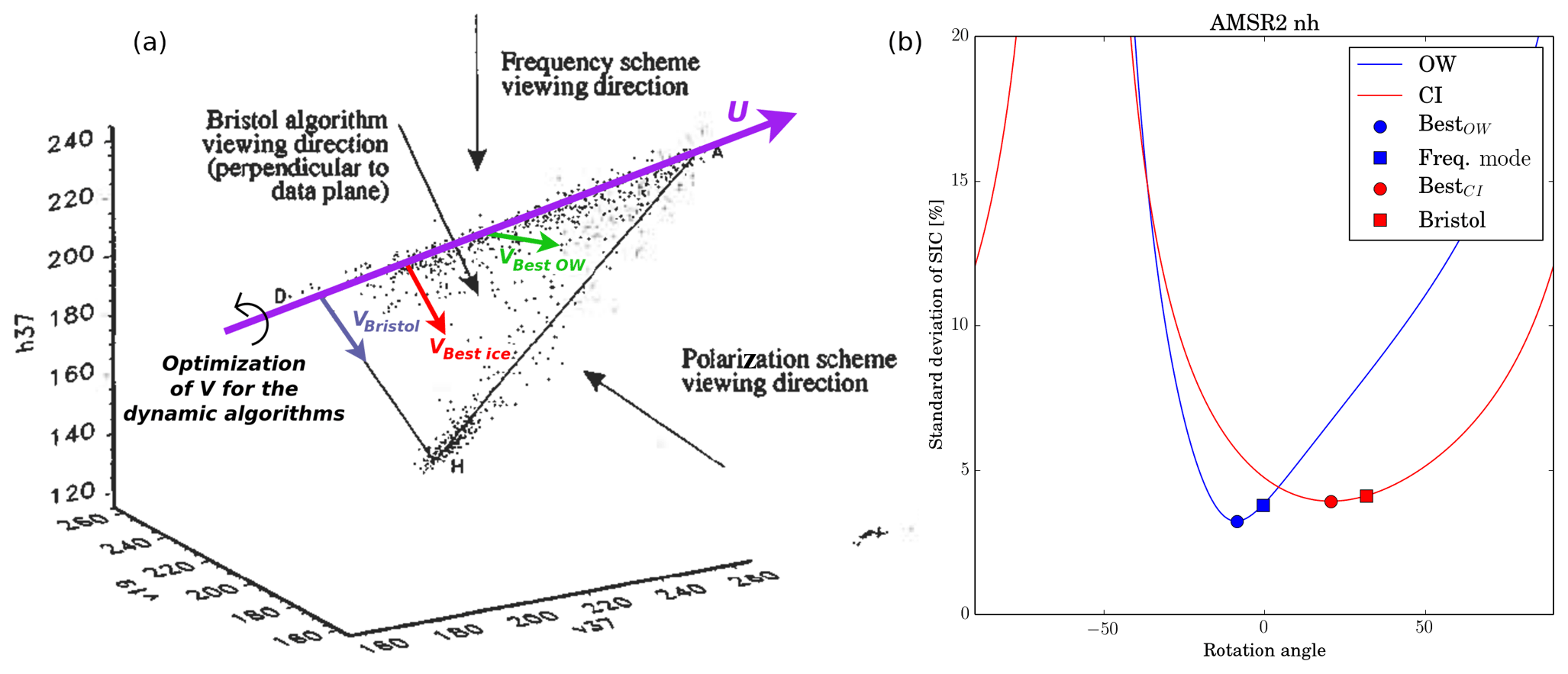
Fig. 4 Three-dimensional diagram of open-water (H) and closed-ice (ice line between D and A) brightness temperatures in a KUKA configuration (Ku-V, Ka-V, Ka-H space) (black dots). The original figure is from Smith [1996]. The direction U (violet, sustained by unit vector \(\vec{u}\)) is shown, and vectors \(\vec{v}_{Bristol}\) (blue), \(\vec{v}_{BestIce}\) (red), and \(\vec{v}_{BestOW}\) (green) are added, as well as an illustration of the optimization of the direction of \(\theta_v\) around the ice-line. (b) Evolution of the SIC algorithm accuracy for open-water (blue) and closed-ice (red) training samples as a function of the rotation angle \(\theta_v\) in the range \([-90^{\circ};+90^{\circ}]\). Square symbols indicate the \(\theta_v\) and accuracy for the Bootstrap Frequency Model (BFM) algorithm and the Bristol (BRI) algorithms. Disk symbols locate the optimized algorithm. Figure reproduced from Lavergne et al. [2019].

The optimization of \(\theta_v\) values uses a Quaternion rotation notation in 3 dimensions. A brute-force approach is chosen where all \(\theta_v\) values in the range \([-90^{\circ};+90^{\circ}]\) are tested with a step of \(1^{\circ}\).

In higher dimensions (\(n>3\)), the contraint in eq. (9) leaves (\(n-2 >= 2\)) degrees of freedom, which requires other optimization approaches than the brute-force strategy we adopt in 3 dimensions. Such higher dimensions SIC algorithms are not envisaged for the CIMR Level-2 SIC product.

Two uncertainty-reduction techniques

Two techniques have been deployed in the EUMETSAT OSI SAF and ESA CCI Sea Ice Concentration processing chains to reduce the SIC retrieval uncertainty:

1. atmospheric correction of the brightness temperature using an RTM;

2. using an ice-curve instead of the ice-line.

The atmospheric correction of TB was first introduced by Andersen et al. [2006] and later refined by Tonboe et al. [2016] and Lavergne et al. [2019] (Sect. 3.4.1). These authors used a RTM (typically those of Wentz [1997]) and auxiliary fields from Numerical Weather Prediction models (e.g. T2m, wind speed, total columnar water vapour, etc…) to correct TBs for the contribution of the atmosphere and ocean surfaces to the TOA signal. The effect in reducing SIC uncertainty is noticeable for algorithms using only Ku-, Ka- or W-band imagery (Fig. 6, Ivanova et al. [2015]) but not so much for algorithms using C-band imagery. The RTM-based correction step has most impact over low SIC areas, and no effect over consolidated 100% SIC areas. While mature, the technique requires a more complex flow-diagram and e.g. an internal iteration loop to implement the RTM-based correction. We do not include this correction step in this version of the ATBD, but it could be included later.

To use an ice-curve instead of an ice-line was first introduce in Lavergne et al. [2019] (Sect. 3.4.2). This was required for algorithms relying on Ku- and Ka-band imagery only to compensate for the difference in depth of the emitting-layer at these two microwave frequencies. The correction had most impact in the Arctic winter months where un-corrected SICs were underestimated in Multiyear ice regions north for Greenland and the Canadian Arctic Archipelago. While C- and Ku-band also have different emitting-layer depth, the impact on CKA SIC is not expected to be large because of the large dynamic range between open water and ice TBs at C-band, and the low sensitivity of C-band to different sea-ice type. For the KUKA configuration, the ice-curve technique would be required, on the other end the main use of KUKA SICs in the CIMR Level-2 product is to pan-sharpen the CKA estimates, so that regional biases in KUKA should not be critical. Since KA SICs use one microwave frequency only, there should not be the need for the ice-curve technique. Implementing an ice-curve instead of an ice-line adds complexity to the processing algorithm and in this version of the ATBD is is left out.

Note

The RTM-based correction and ice-curve techniques are not included in this version of the ATBD, but could be included later if deemed necessary (they are mature techniques but add complexity and dependence to auxiliary data sources).

An hybrid SIC algorithms

As introduced above, a 2-dimensional algorithm (like in the KA configuration) can only be tuned in terms of tie-points \(<\vec{T}^W>\) and \(<\vec{T}^I>\) and \(\vec{u}\) (that itself imposes \(\vec{v}\)). Eq. (2) is used directly to compute SIC from \(\vec{T}\).

For 3-dimensional algorithms like CKA and the KUKA, however, we can tune an algorithm that performs best over the low SIC range (noted \(C_{BestOW}\) or \(C_{OW}\)) and another algorithm that performs best over the high SIC range (noted noted \(C_{BestIce}\) or \(C_{CI}\)). In order to compute a single SIC value for a given \(\vec{T}\), we design an hybrid SIC algorithm that combines \(C_{OW}\) and \(C_{CI}\) linearly:

(10)\[\begin{split} C(\vec{T}) = w_{OW} \times C_{OW}(\vec{T}) + (1 - w_{OW}) \times C_{CI}(\vec{T}) \\ \end{split}\]

with

(11)\[\begin{split} w_{OW} = \left \{\begin{array}{c} 1 \textrm{ for } C_{OW}(\vec{T}) < 0.7 \\ 0 \textrm{ for } C_{OW}(\vec{T}) > 0.9 \\ \frac{C_{OW}(\vec{T}) - 0.7}{0.2} \textrm{ for } C_{OW}(\vec{T}) \in [0.7;0.9] \\ \end{array} \right. \end{split}\]

Eq. (10) and (11) are used to compute a single SIC value from an input \(\vec{T}\). This involves eq. (2) twice (once for \(C_{OW}(\vec{T})\) and once for \(C_{CI}(\vec{T})\)). The same weighting equation in eq. (10) is used to combine the uncertainty estimates (variances) \(\Sigma_C\) of \(C_{OW}\) and \(C_{CI}\) (computed using eq. (4)).

To summarize, SICs in the CKA and KUKA channels combinations are computed using eq. (10) while SICs in the KA channel combination are computed using eq. (2) directly.

Open Water Filter (OWF), thresholding, and climatology masking of SIC

The SIC algorithms described above will return non-zero (positive and negative) SIC values over over open water (0% SIC), even far away from the ice edge. This is because the algorithms are mostly linear-combinations of the brightness temperatures, and the variability of TB around the open water tie-point. In the high SICs range, the algorithms above will sometimes return SIC values above 100% SIC for the same reason.

Historically, these noisy, non-physical SIC values have been removed from the SIC products accessed by the users. Two common filtering techniques have been applied:

1. Open Water Filtering (OWF) (aka Weather Filtering);

2. Thresholding at 100% and 0% SIC;

3. Climatology masking.

Open Water Filter

The OWF is a filter that detects where the ocean is most probably free for ice, and sets the SIC value to 0% SIC in the final product. This filter is needed to get exactly 0% SIC over large ocean areas away from the ice cover. Historically, OWFs have been based on the Ku- and Ka-band channels, sometimes also 22.2 GHz. It generally involved so-called ‘Gradient Ratio’ GR values.

In the CIMR Level-2 SIC algorithm, we follow recent developments at the EUMETSAT OSI SAF and rather use a normalized version of the DAL metric (eq. (8)) as the basis for the OWF. The normalization of DAL involves SIC, a tie-point for First-Year Ice FYI and a “low-weather” (LW) tie-point:

(12)\[ d_{OWF}=d−((1−SIC) \times \vec{u} \cdot <\vec{T}^{LW}> + SIC \times \vec{u} \cdot <\vec{T}^{FYI}>) \]

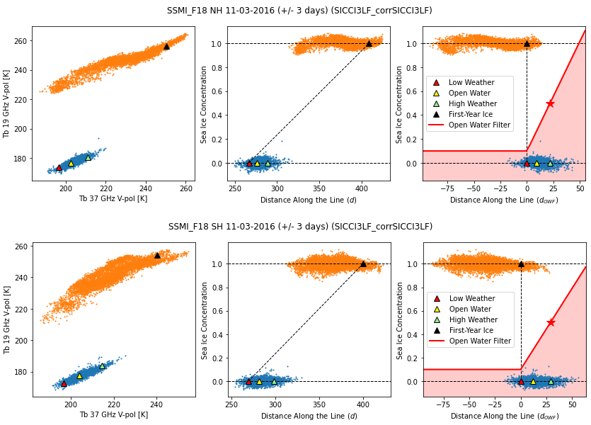
Fig. 5 Example use of \(d\) and \(d_{OWF}\) for Open Water Filtering with the SSMIS mission. Top row for the Arctic, bottom row for the Southern Ocean. Panels from left to right show the Tb samples (small dots) of 0% SIC (blue) and 100% SIC (orange) in a (x:37v,y:19v) space (left panel), (x:\(d\), y:SIC) space (middle panel), and (x:\(d_{OWF}\),y:SIC) space (right panel). Tie-points (triangles) for Open Water (yellow), Low Weather (red), High Weather (green), and First-Year Ice (black) are also reported, as well as the domain detected as Open Water by the Open Water Filter (red area in right panel).

Fig. 5 illustrates how the clusters of 0% and 100% SIC conditions are distributed in three 2D domain relevant for the Open Water Filter. The left-most panels are in the (x:37v, y:19v) Tb space that sustains the traditional Weather Filter through the use of a Gradient Ratio test. The middle panels show the same data in the (x:\(d\), y:SIC) space, to illustrate the intermediate step in the coordinate transform from the left-most to the right-most panels and locate the LW nad FYI tie-points. In the right-most panels, data points are plotted in the (x:\(d_{OWF}\),y:SIC) space that sustains the OWF in the CIMR Level-2 SIC ATBD. The (x:\(d_{OWF}\),y:SIC) space is built so that the intermediate SIC conditions will mostly fall onto and to the left of the (LW, FYI) line (vertical at x=0 in this 2D space).

In this space, the OWF is implemented with two binary tests (see red area in the right-most panels of Fig. 5):

(13)\[\begin{split} \left \{\begin{array}{c} SIC \le 0.1 \\ SIC \le 0.1 + (0.5 – 0.1) \times \frac{d_{OWF}}{d_{HW}} \\ \end{array} \right. \end{split}\]

In eq. (13), \(d_{HW}\) is a point in the (\(d_{OWF}\), SIC) space corresponding to “heavy weather contamination point” at the 95% percentile of the \(d_{OWF}\) values. Eq. (13) detect as water all TA samples that fall below the line going through points (x:0,y=0.1) and (x:\(d_{HW}\),y:0.5) (the latter marked with a red star on Fig. 5).

TB observations that fulfill any of the two conditions in eq. (13) (Test1 OR Test2) are flagged (OWF=True) as “probably open water”, and their SIC is set to 0% in the final Level-2 product file. This filtering is recorded in the status flags, and the “raw” (un-filtered) SICs are also kept in a dedicated variable of the Level-2 product file for expert users (e.g. Data Assimilation).

Thresholding at 100% and 0% SIC

The OWF described in Open Water Filter will generally detect all open water areas in the polar regions, and set their SIC to exactly 0%. By construction, the OWF does not modify the SIC over ice-infested regions. As a results, the SIC field after OWF still has some non-physical values larger than 100%. These values are thresholded to exactly 100%, and the original “raw” values are kept in a dedicated variable of the Level-2 product file.

Although all of them should have been removed by the OWF, potential remaining negative SICs are also thresholded to exactly 0% SIC, and the original “raw” values are kept in a dedicated variable of the Level-2 product file.

Climatology masking

High water vapour content in the tropics can fool the SIC algorithms in returning high SIC values. A monthly varying maximum sea-ice climatology mask is applied to the L1B swath to only compute the Level-2 SICs in the polar regions. Field-of-views outside the maximum climatology mask are either removed from the Level-2 product file, or set to 0% SIC.

Enhanced-resolution SICs using pan-sharpening

The sections above described generically how intermediate SIC fields can be prepared from different channel combinations of CIMR’s imagery (CKA, KUKA, KA). As a result of the input channels, these intermediate SIC fields will have different spatial resolution, and different expected accuracy (see Table 4). The next step in the processing of CIMR Level-2 SIC product is to combine these intermediate SIC fields using a pan-sharpening approach, to obtain final SIC fields that have both high resolution and high accuracy (see Table 5 and Fig. 3).

Pan-sharpening techniques were introduced for improving the spatial resolution of high-resolution optical imagery missions - such as SPOT - in the 1980s. This type of mission typically offered a pan-chromatic imagery band with high spatial resolution (but covering a broad range of wavelengths) and multi-spectral imagery (narrower bandwidth but lower spatial resolution because less photons are recorded). Pan-sharpening techniques emerged for combining the fine details of the pan-chromatic imagery with the information content of the multi-spectral imagery to provide high-resolution multi-spectral imagery. Nowadays many pan-sharpening techniques exist for many missions (see e.g. a review in Meng et al. [2019]} or Dadrass Javan et al. [2021]).

In the field of sea-ice concentration monitoring from passive microwave radiometer data, pan-sharpening has been used recently (e.g. in Ludwig et al. [2019] and Kilic et al. [2020]), noting the early work of Kloster [1996] with the NORSEX algorithm of Svendsen et al. [1987]. A pan-sharpening was also selected in the ESA CCI Sea Ice to produce a 30-years Climate Data Record of SIC.

We select a robust and simple pan-sharpening formulation for the CIMR Level-2 SIC product:

(14)\[\begin{split} \begin{array}{lc} C_{ER} &=& \textrm{Remap}_{HR}(C_{LR}) + \Delta_{edges} \\ &=& \textrm{Remap}_{HR}(C_{LR}) + ( C_{HR} - C_{HR, blurred} ) \\ \end{array} \end{split}\]

In Eq. (14), suffix “ER” refers to enhanced resolution (the final SIC), “LR” to “low resolution” (the SIC to be pan-sharpened), and “HR” to “high resolution” (the SIC used as sharpener). Eq. (14) also involves \(C_{HR, blurred}\) which is C_{HR} blurred to the spatial resolution of \(C_{LR}\). The quantity \(( C_{HR} - C_{HR, blurred})\) is sometimes referred to as a \(\Delta_{edges}\) as it takes small values everywhere but in the regions where \(C_{HR}\) exhibits sharp gradients (e.g. in the MIZ). The \(\textrm{Remap}_{HR}\) operator remaps the location (only the location, not the resolution) of \(C_{LR}\) to those of \(C_{HR}\) to enable adding the two fields together. The resulting SIC field, \(C_{ER}\) is thus at the locations of \(C_{HR}\), with the spatial resolution of \(C_{HR}\) and the accuracy of \(C_{LR}\) (if the pan-sharpening works perfectly).

To the best of our knowledge, the CIMR Level-2 SIC product is the first time the pan-sharpening technique will be used in swath projection for passive microwave SIC retrieval (previous investigations have been deploying the technique on Earth gridded fields).

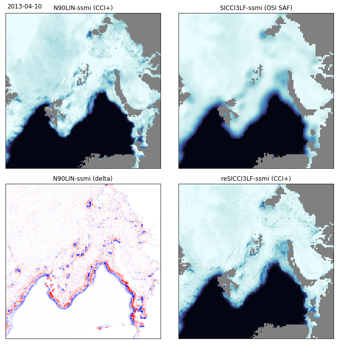
Fig. 6 Illustration of the pan-sharpening technique using SSM/I data in the ESA CCI Sea Ice project (CCI+ Phase 1). The example is for the Arctic on 10th April 2013. Top-left: \(C_{HR}\) (using the near-90 GHz imagery of SSM/I), top-right: \(C_{LR}\) (using a KUKA configuration), bottom-left: \(\Delta_{edges}\) from eq. (14), and bottom-right: the resulting \(C_{ER}\). In this case, \(C_{LR}\) and \(C_{HR}\) had been remapped onto a common 12.5 km EASE2 grid.

Fig. 6 gives an illustration of the resolution enhancement capability of the pan-sharpening technique with the SSM/I mission. In that case, the “LR” SIC was from a KUKA configuration, and the “HR” SIC from using W-band (85.5 GHz) imagery. Transposed to CIMR, a candidate “LR” would be from CKA and “HR” from KA.

At this stage, we cannot foresee what is the combination of intermediate SICs that will achieve best results (in terms of resolution and accuracy) for the CIMR Level-2 SIC product. We thus write this ATBD considering several options for SIC fields in the final Level-2 product file (Fig. 3). These candidate combinations are listed in Table 5.

CIMR Level-1b re-sampling approach

The CIMR Level-2 SIC algorithm involves re-sampling and re-mapping at two stages. The Level-1b brightness temperature samples must be remapped on common location and resolution before applying the CKA, KUKA, and KA algorithms (Fig. 3). At a later stage, the intermediate SICs \(C_{CKA}\), \(C_{KUKA}\), and \(C_{KA}\) must be re-sampled and re-mapped as part of the pan-sharpening step (Enhanced-resolution SICs using pan-sharpening).

At the time of writing, the exact method for re-sampling and re-mapping is not defined. The method might depend on which algorithm is to be applied. For example, the CKA algorithm might benefit from a Backus-Gilbert approach that takes advantage of the overlap of C-band FoVs. On the other hand, KUKA and KA do not involve much overlap between neighbouring FoVs and can thus probably be handled with simpler methods.

Algorithm Assumptions and Simplifications

There are several assumptions and simplifications embedded in the selected algorithm. We describe the main ones below.

Linear scaling of TB with SIC

The basis for most SIC algorithms (including the one selected here) is that an increase in SIC will result in an increase in observed TB. This assumes that the atmosphere is transparent which is mostly the case at polar latitudes for the CIMR frequencies. If the atmosphere is not transparent enough, corrections based on RTM can be used to return to a state where the basis linearity hypothesis is valid.

Large-scale validity of the tie-points

Tie-points are TB values that are characteristics of pure surface (e.g. OW, FYI, etc…) These are typically defined once for all, but can also be adapted on a daily basis as is done in the OSI SAF processing chains. Irrespective of their update frequency, the tie-points are then used for all TB observations in a specific hemisphere, irrespective of the sub-region observed. The tie-points are considered to capture the average sea ice conditions, but regional variability in emissivity exist, and can lead to regional over/under-estimation of the SIC. Region-specific tie-points might be required for monitoring ice on fresh or brackwish waters.

Under-estimation of thin sea ice

Due to many factors (including smooth surface, absence of snow, brine content) concentration of thin sea-ice (<30 cm) is underestimated by most of the PMW SIC algorithms [Cavalieri, 1994]. A complete, 100 % cover of thin sea ice will be retrieved with a lower concentration, depending on the thickness and the microwave frequencies used in the algorithm [Ivanova et al., 2015]. This underestimation is largest for lower frequencies such as L- or C-band.

Land spill-over

The radiometric signature of land is similar to that of sea ice at the wavelengths used for estimating the SIC. Because of the large footprints and the relatively high brightness temperatures of land and ice compared to water, the land signature “spills” into the coastal zone open water and it will falsely appear as intermediate concentration ice.

This land-spillover effect can be partly corrected by estimating the fractional contribution of land surface to each Level-1B sample or FoV. However, coastal correction procedures are not perfect, and some false sea ice might remain along some coastlines and in fjords.