Performance Assessment

Level-2 Sea Ice Drift (SID) algorithm for CIMR

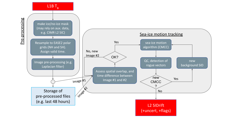
This notebook implements a prototype for a Level-2 SIED algorithm for the CIMR mission.

We refer to the corresponding ATBD and especially the Baseline Algorithm Definition.

In particular, the figure below illustrates the overall concept of the processing:

Settings

Imports and general settings

# Paths

# Getting the path of the notebook (NOTE: not totally safe)
# The paths assume that there is an umbrella CIMR directory (of any name) containing SeaIceDrift_ATBD_v2/ ,
# the CIMR Tools/ directory, and a directory data/L1B/ containing the L1B data, and data/conc/ containing
# a concentration file.
# Additionally, this code expects that the CIMR L2 Sea Ice Drift algorithm notebook has been run, to create
# the drift file
import os
cpath = os.path.join(os.getcwd(), '../..')
algpath = os.path.join(cpath, 'SeaIceDrift_ATBD_v2/algorithm/src_sied')
driftpath = os.path.join(cpath, 'data/icedrift')
figpath = os.path.join(cpath, 'data/figs')

# Imports

import sys
import math
import numpy as np
import numpy.ma as ma
from netCDF4 import Dataset
from matplotlib import pylab as plt
import matplotlib.ticker as mticker
from mpl_toolkits.axes_grid1.axes_divider import make_axes_locatable
import matplotlib.cm as cm
import cmocean
import cartopy
import cartopy.crs as ccrs
from pyresample import parse_area_file

# Local modules contain software code that implement the SIED algorithm
if algpath not in sys.path:
    sys.path.insert(0, algpath)

# Plot settings

import matplotlib
matplotlib.rc('xtick', labelsize=10) 
matplotlib.rc('ytick', labelsize=10) 
matplotlib.rcParams.update({'font.size': 12})
matplotlib.rcParams.update({'axes.labelsize': 12})

font = {'family' : 'sans',
        'weight' : 'normal',
        'size'   : 12}

matplotlib.rc('font', **font)

cmap = cm.viridis

gridtype = 'ease'
gridout = '{}-ease2-250'
# Some region parameters hard-coded to show only the relevant region
# Overall shape of input grid (4320, 4320)
slo = (200, 290, 200, 290)

# EASE plotting region
lon_min = -15
lon_max = 95
lat_min = 74
lat_max = 90

# Settings for gridlines
lon_step = 10
lat_step = 5

plotfigs=True

Parametrize the run

User-set parameters for the running of the whole notebook

hemi = 'nh'

test_card = "radiometric"

griddeffile = os.path.join(algpath, 'grids_py.def')

ncfile = os.path.join(driftpath, 'cimr_devalgo_l2_sid_{}_{}.nc'.format(gridout.format(hemi), test_card))

pixshx = 3
pixshy = 4

Simple Performance Assessment

A simple performance assessment is conducted here for the prototype SID algorithm (see notebooks for pre-processing and algorithm) run on the Radiometric scene. The SID algorithm requires two scenes, with a displacement between them. We thus created a second gridded file by applying a 24-hour time displacement in the metadata, and a 3-pixel x-displacement and a 4-pixel y-displacement to all pixels. The SID was then calculated using the Continuous Maximum Cross-Correlation method between these two gridded files and is here compared to the shift values applied to create the second gridded file. This validation therefore excludes inaccuracies that may arise from the gridding phase, as well as such technical uncertainties such as geolocation.

The chosen 3-pixel displacement in x over a 24-hour period is equivalent in the 5km input grid to 15km/day ice drift, and 4-pixel displacement in y is equivalent to a 20 km/day ice drift. These are reasonably realistic SID values.

def crs_create(gridtype, hemi):

    # Define grid based on region
    if gridtype == 'polstere':
        if hemi == 'nh':
            plot_proj4_params = {'proj': 'stere',
                                 'lat_0': 90.,
                                 'lat_ts' : 70.,
                                 'lon_0': -45.0,
                                 'a': 6378273,
                                 'b': 6356889.44891}
            plot_globe = ccrs.Globe(semimajor_axis=plot_proj4_params['a'],
                                    semiminor_axis=plot_proj4_params['b'])
            plot_crs = ccrs.NorthPolarStereo(
                central_longitude=plot_proj4_params['lon_0'], globe=plot_globe)
        else:
            plot_proj4_params = {'proj': 'stere',
                                 'lat_0': -90.,
                                 'lat_ts' : -70.,
                                 'lon_0': 0.,
                                 'a': 6378273,
                                 'b': 6356889.44891}
            plot_globe = ccrs.Globe(semimajor_axis=plot_proj4_params['a'],
                                    semiminor_axis=plot_proj4_params['b'])
            plot_crs = ccrs.SouthPolarStereo(
                central_longitude=plot_proj4_params['lon_0'], globe=plot_globe)
    elif gridtype == 'ease':
        if hemi == 'nh':
            plot_crs = ccrs.LambertAzimuthalEqualArea(central_longitude=0,
                                                      central_latitude=90,
                                                      false_easting=0,
                                                      false_northing=0)
        else:
            plot_crs = ccrs.LambertAzimuthalEqualArea(central_longitude=0,
                                                      central_latitude=-90,
                                                      false_easting=0,
                                                      false_northing=0)
    else:
        raise ValueError("Unrecognised region {}".format(region))

    return(plot_crs)

# Reading NetCDF file

def nc_read(ncfile, var, skip=None, procfmt=False):

    ncdata = {}

    if isinstance(var, list):
        v = var[0]
    else:
        v = var

    # Reading from the NetCDF file
    with Dataset(ncfile, 'r') as dataset:

        try:
            ncdata['fv'] = dataset.variables[v].__dict__['_FillValue']
        except:
            pass

        if isinstance(var, list):
            varlist = var
        else:
            varlist = [var]
        for item in varlist:
            vardata = dataset[item][:]
            if len(vardata.shape) == 3:
                if skip:
                    vardata = vardata[0, ::skip, ::skip]
                else:
                    vardata = vardata[0, :, :]
            else:
                if skip:
                    vardata = vardata[::skip, ::skip]
                else:
                    vardata = vardata[:, :]

            # This is for reducing flags to the lowest integers
            if var in ['statusflag', 'status_flag', 'flag']:
                vardata = np.asarray(vardata, float) + 100
                uniques = np.unique(vardata)
                uniques = uniques[np.logical_not(np.isnan(uniques))]
                for newval, origval in enumerate(uniques):
                    vardata[vardata == origval] = newval
                ncdata['sf_labs'] = [str(int(u - 100)) for u in uniques]

            # NOTE: Be very careful with the fill value here. Trying to
            # use ncdata['fv'] as the fill_value for a status array such
            # as 'flag' means that flag values of 0 (i.e. nominal) are
            # masked out
            if 'fv' in ncdata.keys() and item not in ['statusflag',
                                                      'status_flag', 'flag']:
                ncdata[item] = ma.array(vardata, fill_value=ncdata['fv'])
            else:
                ncdata[item] = ma.array(vardata)

            if var in ['statusflag', 'status_flag', 'flag']:
                ncdata[item].mask = None
            else:
                ncdata[item].mask = ncdata[item].data == ncdata[item].fill_value

        if skip:
            ncdata['lon'] = dataset.variables['lon'][::skip, ::skip]
            ncdata['lat'] = dataset.variables['lat'][::skip, ::skip]
        else:
            ncdata['lon'] = dataset.variables['lon'][:]
            ncdata['lat'] = dataset.variables['lat'][:]

        # Try fetching time info
        try:
            try:
                d0 = datetime.strptime(dataset.start_date,'%Y-%m-%d %H:%M:%S')
                d1 = datetime.strptime(dataset.stop_date,'%Y-%m-%d %H:%M:%S')
            except:
                try:
                    d0 = datetime.strptime(dataset.start_date_and_time,
                                           '%Y-%m-%dT%H:%M:%SZ')
                    d1 = datetime.strptime(dataset.end_date_and_time,
                                           '%Y-%m-%dT%H:%M:%SZ')
                except:
                    d0 = datetime.strptime(dataset.time_coverage_start,
                                           '%Y-%m-%dT%H:%M:%SZ')
                    d1 = datetime.strptime(dataset.time_coverage_end,
                                           '%Y-%m-%dT%H:%M:%SZ')
            d0_00 = datetime.combine(d0.date(),time(0))
            d1_00 = datetime.combine(d1.date(),time(0))
            ncdata['sdate'] = d0_00
            ncdata['edate'] = d1_00
            ncdata['tspan_hours'] = (d1_00 - d0_00).total_seconds() / (60.*60.)
        except:
            pass

        ncdata['time'] = dataset.variables['time'][0]

    return ncdata

# Reading in the data

varlist = ['driftX', 'driftY', 'status_flag']
iddata = nc_read(ncfile, varlist, skip=None, procfmt=True)

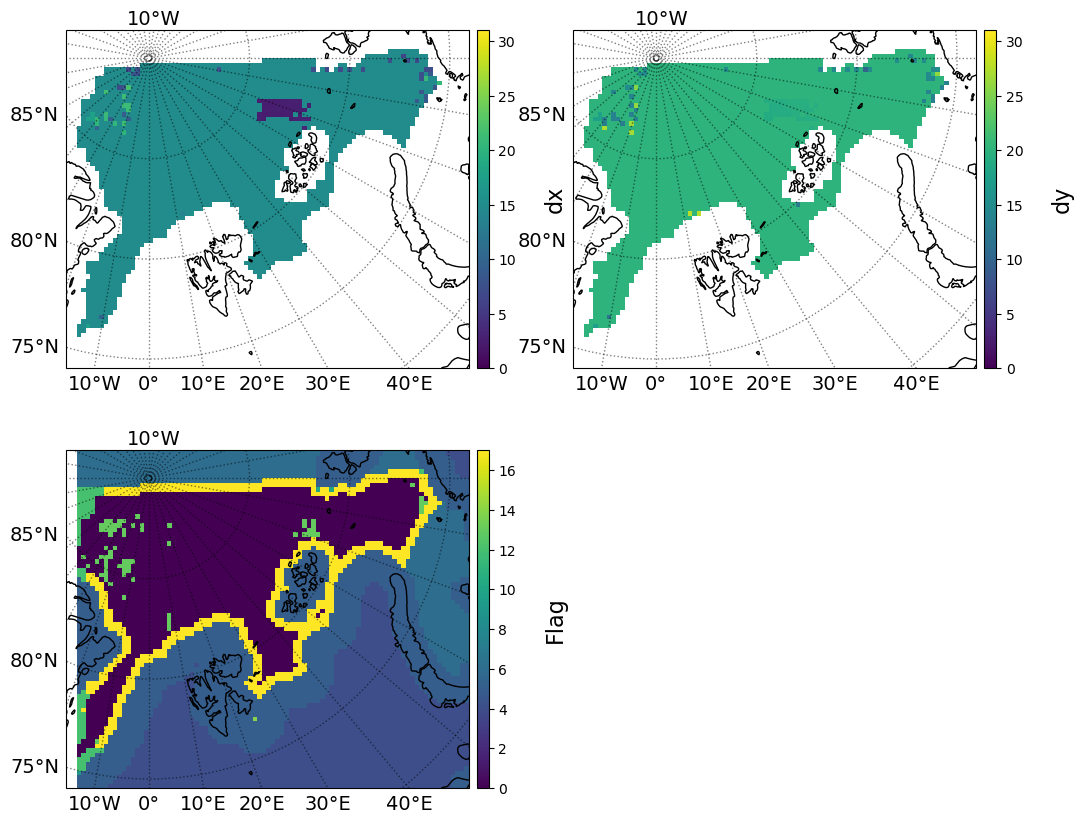
# Plotting the ice drift
# Modified from the SeaSurfaceTemperature_ATBD_v2, by Emy Alerskans

# Drift data
xydata = {'dx': iddata['driftX'], 'dy': iddata['driftY']}
flag = iddata['status_flag']
limminxy = np.nanmin([np.nanmin(a) for a in xydata.values()])
limminxy = limminxy - 0.1 * abs(limminxy)
limmaxxy = np.nanmax([np.nanmax(a) for a in xydata.values()])
limmaxxy = limmaxxy + 0.1 * abs(limmaxxy)
limminflag = np.nanmin(flag)
limmaxflag = np.nanmax(flag)

# Output lat/lons
og = gridout.format(hemi)
out_area_def = parse_area_file(griddeffile, og)[0]
olons, olats = out_area_def.get_lonlats()

# Coordinate reference systems
plot_crs = crs_create(gridtype, hemi)
pc = ccrs.PlateCarree()

# Plotting drift
fig = plt.figure(figsize=[12, 10])
for i, var in enumerate(list(xydata.keys())):
    ax = fig.add_subplot(2, 2, i+1, projection=plot_crs)
    im = ax.pcolormesh(olons[slo[0]:slo[1], slo[2]:slo[3]], olats[slo[0]:slo[1], slo[2]:slo[3]], 
                       xydata[var][:][slo[0]:slo[1], slo[2]:slo[3]], transform=pc,
                       cmap=cmap, vmin=0, vmax=math.ceil(limmaxxy))
    ax.coastlines()
    ax.set_extent([lon_min, lon_max, lat_min, lat_max])
    gl = ax.gridlines(crs=ccrs.PlateCarree(), draw_labels=True, linewidth=1, color='k', alpha=0.5, linestyle=':')
    gl.top_labels = False
    gl.right_labels = False
    gl.xlocator = mticker.FixedLocator(np.arange(-180, 180, lon_step))
    gl.ylocator = mticker.FixedLocator(np.arange(-90, 90, lat_step))
    gl.xlabel_style = {'size': 14}
    gl.ylabel_style = {'size': 14}
        
    # Colourbar
    divider = make_axes_locatable(ax)
    cax = divider.append_axes("right", size="3%", pad="2%", axes_class=plt.Axes)
    cb = fig.colorbar(im, cax=cax)
    cb.set_label(label=var, fontsize=16, labelpad=20.0)
    cb.ax.set_ylim(0, math.ceil(limmaxxy))
    

# Status flags
ax = fig.add_subplot(2, 2, 3, projection=plot_crs)
im = ax.pcolormesh(olons[slo[0]:slo[1], slo[2]:slo[3]], olats[slo[0]:slo[1], slo[2]:slo[3]], 
                    flag[:][slo[0]:slo[1], slo[2]:slo[3]], transform=pc,
                    cmap=cmap, vmin=limminflag, vmax=limmaxflag)
ax.coastlines()
ax.set_extent([lon_min, lon_max, lat_min, lat_max])
gl = ax.gridlines(crs=ccrs.PlateCarree(), draw_labels=True, linewidth=1, color='k', alpha=0.5, linestyle=':')
gl.top_labels = False
gl.right_labels = False
gl.xlocator = mticker.FixedLocator(np.arange(-180, 180, lon_step))
gl.ylocator = mticker.FixedLocator(np.arange(-90, 90, lat_step))
gl.xlabel_style = {'size': 14}
gl.ylabel_style = {'size': 14}
        
# Colourbar
divider = make_axes_locatable(ax)
cax = divider.append_axes("right", size="3%", pad="2%", axes_class=plt.Axes)
cb = fig.colorbar(im, cax=cax)
cb.set_label(label="Flag", fontsize=16, labelpad=20.0)
cb.ax.set_ylim(limminflag, limmaxflag)
        
if plotfigs:
    plt.savefig(os.path.join(figpath, 'dxdy.png'))
plt.show()

print("\
FLAG VALUES \n\
Unprocessed pixel                              -1\n\
Nominal                                        0\n\
Outside image border                           1\n\
Close to image border                          2\n\
Pixel center over land                         3\n\
No ice                                         4\n\
Close to coast or edge                         5\n\
Close to missing pixel                         6\n\
Close to unprocessed pixel                     7\n\
Icedrift optimisation failed                   8\n\
Icedrift failed                                9\n\
Icedrift with low correlation                  10\n\
Icedrift calculation took too long             11\n\
Icedrift calculation refused by neighbours     12\n\
Icedrift calculation corrected by neighbours   13\n\
Icedrift no average                            14\n\
Icedrift masked due to summer season           15\n\
Icedrift multi-oi interpolation                16\n\
Icedrift calcuated with smaller pattern        17\n\
Icedrift masked due to NWP                     18\n\
")

FLAG VALUES 
Unprocessed pixel                              -1
Nominal                                        0
Outside image border                           1
Close to image border                          2
Pixel center over land                         3
No ice                                         4
Close to coast or edge                         5
Close to missing pixel                         6
Close to unprocessed pixel                     7
Icedrift optimisation failed                   8
Icedrift failed                                9
Icedrift with low correlation                  10
Icedrift calculation took too long             11
Icedrift calculation refused by neighbours     12
Icedrift calculation corrected by neighbours   13
Icedrift no average                            14
Icedrift masked due to summer season           15
Icedrift multi-oi interpolation                16
Icedrift calcuated with smaller pattern        17
Icedrift masked due to NWP                     18

Here the output x- and y-components of drift are plotted. They are close to the 15 km/day in x and 20 km/day in y expected from the input data, except for one patch around 70E, 83N, which the ice drift algorithm has not calculated correctly for the x-direction. This is suspected to be due to the limitations of the Radiometric test card, which has somewhat “blocky” features, and for the next round of algorithm improvements emphasis will be on an improved set of test scenes. These are planned to be created from model data, transformed onto a set of swaths separated in time, and then run through the CIMR data simulator. Therefore these scenes will have the texture expected of satellite observations of sea ice at this resolution, and the algorithm will have more pattern to match.

There is also a region around 20W,86N where the vectors were interpolated and are thus less accurate.

# Plotting the residuals
# Modified from the SeaSurfaceTemperature_ATBD_v2, by Emy Alerskans

pixsize = 5.0
expectedx = pixshx * pixsize
expectedy = pixshy * pixsize
testx = np.full(iddata['driftX'].shape, expectedx)
testy = np.full(iddata['driftX'].shape, expectedy)

testdata = {'dx': testx, 'dy': testy}
resx = iddata['driftX'] - testx
resy = iddata['driftY'] - testy
resdata = {'dx': resx, 'dy': resy}

limminres = np.nanmin([np.nanmin(a) for a in resdata.values()])
limminres = limminres - 0.1 * abs(limminres)
limmaxres = np.nanmax([np.nanmax(a) for a in resdata.values()])
limmaxres = limmaxres + 0.1 * abs(limmaxres)
lim = max([abs(limminres), limmaxres])

fig = plt.figure(figsize=[12, 5])
for i, var in enumerate(list(resdata.keys())):
    ax = fig.add_subplot(1, 2, i+1, projection=plot_crs)
    im = ax.pcolormesh(olons[slo[0]:slo[1], slo[2]:slo[3]], olats[slo[0]:slo[1], slo[2]:slo[3]], 
                       resdata[var][:][slo[0]:slo[1], slo[2]:slo[3]], transform=pc,
                       cmap=cmocean.cm.balance, vmin=-lim, vmax=lim)
    ax.coastlines()
    ax.set_extent([lon_min, lon_max, lat_min, lat_max])
    gl = ax.gridlines(crs=ccrs.PlateCarree(), draw_labels=True, linewidth=1, color='k', alpha=0.5, linestyle=':')
    gl.top_labels = False
    gl.right_labels = False
    gl.xlocator = mticker.FixedLocator(np.arange(-180, 180, lon_step))
    gl.ylocator = mticker.FixedLocator(np.arange(-90, 90, lat_step))
    gl.xlabel_style = {'size': 14}
    gl.ylabel_style = {'size': 14}
        
    # Colourbar
    divider = make_axes_locatable(ax)
    cax = divider.append_axes("right", size="3%", pad="2%", axes_class=plt.Axes)
    cb = fig.colorbar(im, cax=cax)
    cb.set_label(label=var, fontsize=16, labelpad=20.0)
    cb.ax.set_ylim(-lim, lim)
        
if plotfigs:
    plt.savefig(os.path.join(figpath, 'resdxdy.png'))
plt.show()

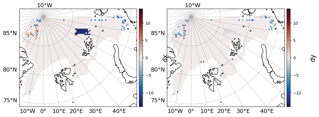
Here the residuals are plotted, and again, the areas in which the algorithm did not fully succeed are highlighted, while most of the field has a well-calculated ice drift.

# Plotting a histogram

minbin = math.floor(limminres)
maxbin = math.ceil(limmaxres) + 1
hbins = list(range(minbin, maxbin, 1))
#step = 0.5
#hbins = [(step * x) + minbin for x in range((int(abs(maxbin - minbin) / step)))]

import matplotlib.transforms as transforms

fig = plt.figure(figsize=(12,5))
ax = {}
c = {}
for i, var in enumerate(list(resdata.keys())):
    ax[i] = fig.add_subplot(1,len(resdata),i+1)    
    ax[i].hist(resdata[var][:].flatten(), bins=hbins)
    ax[i].set_title('{}-drift residuals'.format(var[1:2]), fontsize=12)

    ax[i].text(0.39,0.96, 'BIAS: {:.2f} [km]'.format(np.nanmean(resdata[var])),
        transform=ax[i].transAxes, ha='right', va='top', fontsize='xx-small')
    ax[i].text(0.39,0.90, 'RMSE: {:.2f} [km]'.format(np.nanstd(resdata[var])),
        transform=ax[i].transAxes, ha='right', va='top', fontsize='xx-small')

if plotfigs:
    plt.savefig(os.path.join(figpath, 'hist_res.png'))
plt.show()

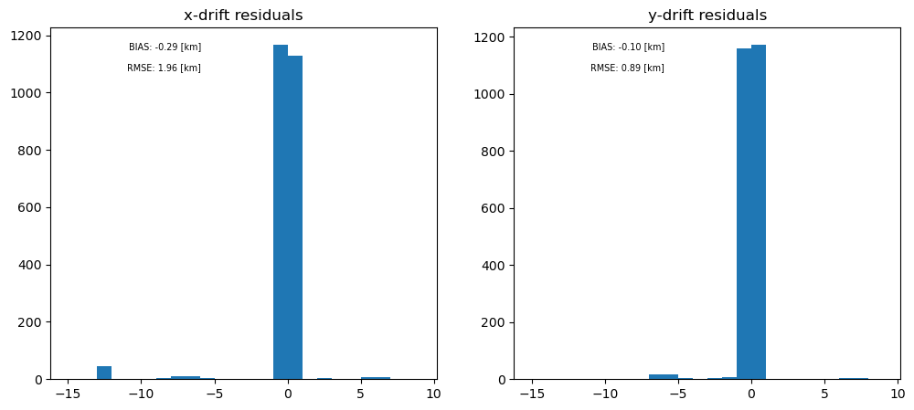
The histograms of residuals are shown here. The RMSE for this artifical data is below the target value of 2.6 km/day from the MRD, ~2 km (lower for y-direction). The bias is also reasonably low, -0.3 km (lower for y-direction). The mismatch between x and y here is due to the fact that the bulk of the error comes from the one single patch that the algorithm did not calculate well in the x-direction. It is predicted that this will not be an issue with more realistic test scenes.

In addition, the residuals here are not expected to be accurate, due to the lack of natural features in the test card, and the fact that the second gridded image was exactly the first gridded image but with a shift. We will be able to characterise likely residuals better with the more realistic test cards we are planning to use in L2PAD.