Preprocessing#
Level-2 Sea Ice Drift (SID) algorithm for CIMR#
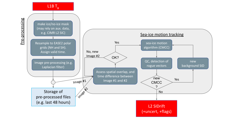
This notebook implements a prototype for a Level-2 SIED algorithm for the CIMR mission.
We refer to the corresponding ATBD and especially the Baseline Algorithm Definition.
In particular, the figure below illustrates the overall concept of the processing:
Settings#
Imports and general settings
# Paths

# Getting the path of the notebook (NOTE: not totally safe)

# The paths assume that there is an umbrella CIMR directory (of any name) containing SeaIceDrift_ATBD_v2/ ,
# the CIMR Tools/ directory, and a directory data/L1B/ containing the L1B data, and data/conc/ containing
# a concentration file
import os
cpath = os.path.join(os.getcwd(), '../..')
algpath = os.path.join(cpath, 'SeaIceDrift_ATBD_v2/algorithm/src_sied')
toolpath = os.path.join(cpath, 'Tools')
l1bpath = os.path.join(cpath, 'data/L1B')
griddeffile = os.path.join(cpath, 'Overall_ATBD/etc/grids_py.def')

# Creating a directory structure for processing
concpath = os.path.join(cpath, 'data/conc')
icemaskpath = os.path.join(cpath, 'data/icemask')
swathpath = os.path.join(cpath, 'data/swaths')
procpath = os.path.join(cpath, 'data/processing')
driftpath = os.path.join(cpath, 'data/icedrift')
logpath = os.path.join(cpath, 'data/logs')
figpath = os.path.join(cpath, 'data/figs')
for pth in [concpath, icemaskpath, swathpath, procpath, driftpath, logpath, figpath]:
    if not os.path.isdir(pth):
        os.makedirs(pth)
# Imports
from importlib import reload
import sys
import warnings
from datetime import datetime, timedelta
from dateutil.relativedelta import relativedelta
import numpy as np
import xarray as xr
from netCDF4 import Dataset
from matplotlib import pylab as plt
import matplotlib.cm as cm
from pyresample import parse_area_file
from scipy.ndimage import laplace

# Local modules contain software code that implement the SIED algorithm
if algpath not in sys.path:
    sys.path.insert(0, algpath)
from process_ice_mask import process_ice_mask
from cp_and_date_change_iceconc import cp_and_date_change_iceconc

# Prototype re-gridding toolbox to handle the L1B input
if toolpath not in sys.path:
    sys.path.insert(0, toolpath)
from tools import io_handler as io
from tools import collocation as coll
from tools import l2_format as l2
# Plot settings

import matplotlib
matplotlib.rc('xtick', labelsize=10)
matplotlib.rc('ytick', labelsize=10)
matplotlib.rcParams.update({'font.size': 12})
matplotlib.rcParams.update({'axes.labelsize': 12})

font = {'family' : 'sans',
        'weight' : 'normal',
        'size'   : 12}
matplotlib.rc('font', **font)

cmap = cm.viridis
cmapland = matplotlib.colors.ListedColormap(['none', 'grey'])

gridin = '{}-ease2-050'
gridout = '{}-ease2-250'
# Some region parameters hard-coded to show only the relevant region
# Overall shape of input grid (4320, 4320)
sl = (1050, 1400, 1050, 1400)
Parametrize the run#
User-set parameters for the running of the whole notebook. Note that here a helper script is used to copy a starter ice concentration file from the MET Norway thredds server and change the dates in this. The date changes are required due to the sample input file having a date in the future (2028).
hemi = 'nh'
algos = {'KU': {'channels':('tb19v', 'tb19h'), 'target_band':'KU'},
         'KA': {'channels':('tb37v', 'tb37h'), 'target_band':'KA'}}
wbs = list(algos.keys())
fwdbck = ['fw', 'bk']
polarisation = {'V': 0, 'H': 1}
pols = list(polarisation.keys())

test_card = "radiometric"
if test_card == "geometric":
    # DEVALGO's simulated geometric test card
    l1bfn = 'W_PT-DME-Lisbon-SAT-CIMR-1B_C_DME_20230417T105425_LD_20280110T114800_20280110T115700_TN.nc'
elif test_card == "radiometric":
    # DEVALGO's simulated radiometric test card
    l1bfn = 'W_PT-DME-Lisbon-SAT-CIMR-1B_C_DME_20230420T103323_LD_20280110T114800_20280110T115700_TN.nc'

l1bfile = os.path.join(l1bpath, l1bfn)

pdate = datetime.strptime('20280110', '%Y%m%d')
tdate = pdate - relativedelta(years=10)
qdate = pdate + timedelta(days=1)

# Icemask data and output locations
icemaskinputdir = 'https://thredds.met.no/thredds/dodsC/osisaf/met.no/reprocessed/ice/conc_450a_files/{:%Y}/{:%m}'.format(tdate, tdate)
icemaskinputfile = 'ice_conc_{}_ease2-250_cdr-v3p0_{:%Y%m%d}1200.nc'.format(hemi, tdate)
icemaskinput = cp_and_date_change_iceconc(os.path.join(icemaskinputdir, icemaskinputfile), concpath, pdate)

algo_version = '0.1'

pixshx = 3
pixshy = 4
Written a version of https://thredds.met.no/thredds/dodsC/osisaf/met.no/reprocessed/ice/conc_450a_files/2018/01/ice_conc_nh_ease2-250_cdr-v3p0_201801101200.nc to /home/emilyjd/cimr-devalgo/SeaIceDrift_ATBD_v2/algorithm/../../data/conc/ice_conc_nh_ease2-250_cdr-v3p0_202801101200.nc
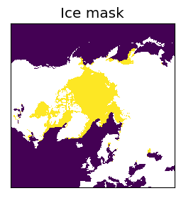
Step 1: Creating and regridding the ice mask#
A land/ocean/ice mask is required to define the areas with ice to the algorithm. This is created from a concentration file, and is stored for future use. Since there can be multiple ice drift calculations per day on different swaths, the mask can be reused once created.
# Creating the ice mask
gridname = gridin.format(hemi)
icemaskname = os.path.join(icemaskpath, 'icemask-multi-{}-{:%Y%m%d}12.nc'.format(gridname, pdate))
if not os.path.isfile(icemaskname):
    # Suppress the proj4 string warning on this
    with warnings.catch_warnings():
        warnings.simplefilter("ignore")
        process_ice_mask(icemaskinput, icemaskpath, griddeffile, gridname)

# Reading in the ice mask
ie_data = Dataset(icemaskname, 'r')
ie = ie_data['ice_edge'][0, :, :]

# And the same for the output grid
gridnameout = gridout.format(hemi)
icemasknameout = os.path.join(icemaskpath, 'icemask-multi-{}-{:%Y%m%d}12.nc'.format(gridnameout, pdate))
if not os.path.isfile(icemasknameout):
    # Suppress the proj4 string warning on this
    with warnings.catch_warnings():
        warnings.simplefilter("ignore")
        process_ice_mask(icemaskinput, icemaskpath, griddeffile, gridnameout)
ie_data_out = Dataset(icemasknameout, 'r')
ieout = ie_data_out['ice_edge'][0, :, :]

# Plotting the ice mask
fig = plt.figure(figsize=(3,3))
ax1 = fig.add_subplot(1,1,1)
c1 = ax1.imshow(ie[:], interpolation = 'none', cmap=cmap)
ax1.set_title("Ice mask")
ax1.xaxis.set_tick_params(labelbottom=False)
ax1.yaxis.set_tick_params(labelleft=False)
ax1.set_xticks([])
ax1.set_yticks([])

# Input landmask
landmask = np.zeros_like(ie)
landmask[ie == 9] = 1

# Output landmask
landmaskout = np.zeros_like(ieout)
landmaskout[ieout == 9] = 1
Step 2: Loading the data#
The L1B data is read in and split into forward and backward scans using software from the Tools/ repository (a prototype CIMR Regridding Toolbox developed in the CIMR DEVALGO study). These forward and backward scans can be used independently in the algorithm in the same way as different channels and polarisations.
# Read the bands needed of the L1B data
reload(io)

tb_dict = {'tb01':'L', 'tb06':'C', 'tb10':'X', 'tb19':'KU', 'tb37':'KA'}
rev_tb_dict = {v:k for k,v in tb_dict.items()}
bands_needed = []
for alg in algos.keys():
    bands_needed += algos[alg]['channels']
bands_needed = list(set([tb_dict[b[:-1]] for b in bands_needed]))

full_l1b = io.CIMR_L1B(l1bfile, selected_bands=bands_needed, keep_calibration_view=True)
# Split into forward / backward scan

l1b = {}
l1b['fw'], l1b['bk'] = full_l1b.split_forward_backward_scans(method='horn_scan_angle')
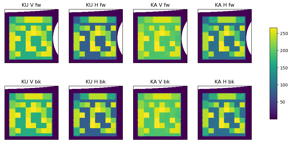
Step 3: Regridding the data#
The horns are interleaved, and then the data is regridded. These are again done with software from Tools/. The ice drift will be calculated individually on 8 fields based on the forward and backward scans, waveband (Ku or Ka), and polarity (V or H). A fine EASE2 grid spacing of 5km is chosen for this regridding.
# Regridding the data

reload(coll)

# Reshaping
l1b_r = {}
for fb in fwdbck:
    l1b_r[fb] = l1b[fb].reshape_interleave_feed()

# Loading the target grid information
gridname = gridin.format(hemi)
new_area_def = parse_area_file(griddeffile, gridname)[0]
new_lons, new_lats = new_area_def.get_lonlats()

# Getting the input lat/lons
lonlats = {}
for ll in ['lon', 'lat']:
    lonlats[ll] = {}
    for fb in fwdbck:
        lonlats[ll][fb] = {}
        for wb in wbs:
            lonlats[ll][fb][wb] = l1b_r[fb].data[wb][ll].data

# Creating data arrays with the V and H layers
what = ('brightness_temperature_v', 'brightness_temperature_h')
params = {'method':'gauss', 'sigmas':25000, 'neighbours':55}
stack_shape = {}
stack = {}
regrid = {}
for fb in fwdbck:
    stack_shape[fb] = {}
    stack[fb] = {}
    regrid[fb] = {}
    for wb in wbs:
        stack_shape[fb][wb] = tuple(list(lonlats['lat'][fb][wb].shape) + [len(what),])
        stack[fb][wb] = np.empty(stack_shape[fb][wb])
        for iw, w in enumerate(what):
            stack[fb][wb][...,iw] = l1b_r[fb].data[wb][w].data
            # Regridding
            # TODO - Add passing of params, currently a nearest-neighbour approach with ROI 15000 is used
            regrid[fb][wb] = coll._regrid_fields(new_lons, new_lats,
                                                 lonlats['lon'][fb][wb], lonlats['lat'][fb][wb], stack[fb][wb])
# Plot regridded

fig = plt.figure(figsize=(12,6))
ax = {}
c = {}
shapelayout = (len(fwdbck), len(wbs) * len(pols))
axindex = 1
for fb in fwdbck:
    for wb in wbs:
        for pol in pols:
            ax[axindex] = fig.add_subplot(*shapelayout, axindex)
            c[axindex] = ax[axindex].imshow(regrid[fb][wb][:, :, polarisation[pol]][sl[0]:sl[1], sl[2]:sl[3]],
                                            interpolation = 'none', origin='lower', cmap=cmap)
            overland = ax[axindex].imshow(landmask[sl[0]:sl[1], sl[2]:sl[3]], interpolation='none',
                                          origin='lower', cmap=cmapland)
            ax[axindex].invert_yaxis()
            ax[axindex].set_title("{} {} {}".format(wb, pol, fb), fontsize=12)
            ax[axindex].xaxis.set_tick_params(labelbottom=False)
            ax[axindex].yaxis.set_tick_params(labelleft=False)
            ax[axindex].set_xticks([])
            ax[axindex].set_yticks([])
            axindex += 1

fig.subplots_adjust(right=0.8)
cbar_ax = fig.add_axes([0.85, 0.25, 0.02, 0.5])
fig.colorbar(c[1], cax=cbar_ax, shrink=0.5)
<matplotlib.colorbar.Colorbar at 0x7fbecd45b220>
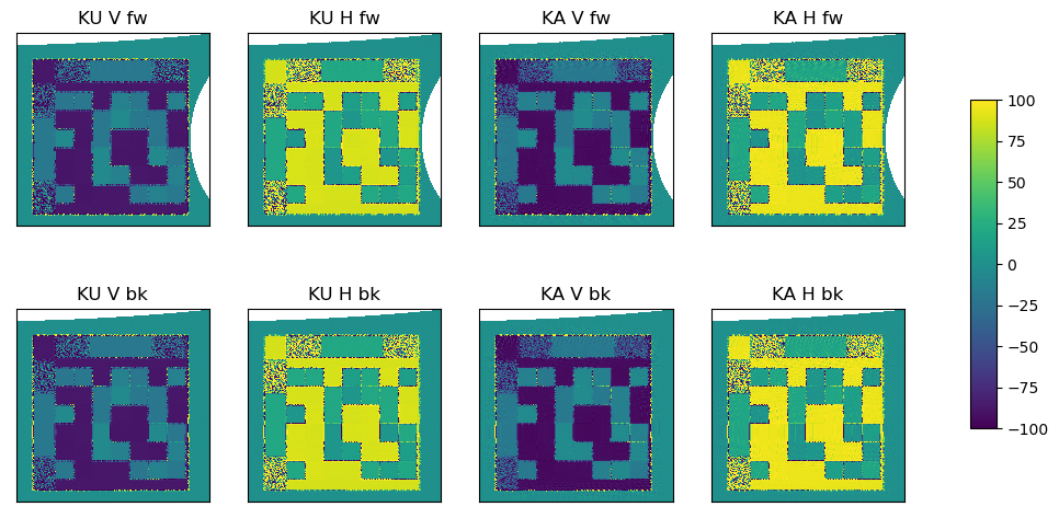
Step 4: Laplacian pre-processing#
Instead of directly using the brightness temperatures in the motion tracking algorithm, the ice features are stabilised and enhanced by applying a Laplacian filter (see ATBD for mathmatical description).
# Replace fill value by NaN and remove mask
def _get_nans(img):
    img_masked = np.ma.asarray(img)
    return img_masked.filled(np.nan)

# Replace NaN by fill value and add mask
def _mask_nans(img):
    return np.ma.masked_invalid(img)

nan = {}
lap = {}
fv = {}
for fb in fwdbck:
    nan[fb] = {}
    lap[fb] = {}
    fv[fb] = {}
    for wb in wbs:
        # Convert fill values to NaNs
        nan[fb][wb] = _get_nans(regrid[fb][wb])
        # Laplacian transform
        lap[fb][wb] = laplace(nan[fb][wb])
        # Converting NaNs to fill values
        fv[fb][wb] = _mask_nans(lap[fb][wb])

# Creating a flag field
#define TCIMAGE_OUTSIDE_GRID              -2
#define TCIMAGE_NODATA                    -1
#define TCIMAGE_OK                         0
#define TCIMAGE_UNPROCESSED                1
#define TCIMAGE_FAILED                     2
flag = {}
for fb in fwdbck:
    flag[fb] = {}
    for wb in wbs:
        flag[fb][wb] = np.zeros_like(fv[fb][wb])
        # Masking where the Laplacian didn't work
        flag[fb][wb][fv[fb][wb].mask] = -1
        # Masking where the land and ocean is
        landocean = np.logical_or(ie == 9, ie == 1)
        flag[fb][wb][landocean] = 1
# Plot Laplacian

vmin = -100
vmax = 100

fig = plt.figure(figsize=(12,6))
ax = {}
c = {}
shapelayout = (len(fwdbck), len(wbs) * len(pols))
axindex = 1
for fb in fwdbck:
    for wb in wbs:
        for pol in pols:
            ax[axindex] = fig.add_subplot(*shapelayout, axindex)
            c[axindex] = ax[axindex].imshow(fv[fb][wb][:, :, polarisation[pol]][sl[0]:sl[1], sl[2]:sl[3]],
                                            interpolation = 'none', origin='lower', cmap=cmap,
                                            vmin=vmin, vmax=vmax)
            overland = ax[axindex].imshow(landmask[sl[0]:sl[1], sl[2]:sl[3]], interpolation='none',
                                          origin='lower', cmap=cmapland)
            ax[axindex].invert_yaxis()
            ax[axindex].set_title("{} {} {}".format(wb, pol, fb), fontsize=12)
            ax[axindex].xaxis.set_tick_params(labelbottom=False)
            ax[axindex].yaxis.set_tick_params(labelleft=False)
            ax[axindex].set_xticks([])
            ax[axindex].set_yticks([])
            axindex += 1

fig.subplots_adjust(right=0.8)
cbar_ax = fig.add_axes([0.85, 0.25, 0.02, 0.5])
fig.colorbar(c[1], cax=cbar_ax, shrink=0.5)
<matplotlib.colorbar.Colorbar at 0x7fbee6a1b340>
Step 5: Writing out the file#
For ice drift, it is not possible to keep the data only internally. Since two gridded files at different timepoints are required to create each gridded map of icedrift vectors, it is necessary to write each gridded swath file to disk so that it can be read in to be compared with other gridded swath files.
# Note: It is deprecated, but the wrapper and C code still expect a input proj4_string, so accept the
# deprecation warning for now.
with warnings.catch_warnings():
    warnings.simplefilter("ignore")
    crs_info = {'proj4_string': new_area_def.proj4_string,
                 'area_id': new_area_def.area_id,
                 'semi_major_axis': 6378137.,
                 'semi_minor_axis': 6356752.31424518,
                 'inverse_flattening': 298.257223563,
                 'reference_ellipsoid_name': "WGS 84",
                 'longitude_of_prime_meridian': 0.,
                 'prime_meridian_name': "Greenwich",
                 'geographic_crs_name': "unknown",
                 'horizontal_datum_name': "World Geodetic System 1984",
                 'projected_crs_name': "unknown",
                 'grid_mapping_name': "lambert_azimuthal_equal_area",
                 'latitude_of_projection_origin': 90.,
                 'longitude_of_projection_origin': 0.,
                 'false_easting': 0.,
                 'false_northing': 0.}
reload(l2)

# Get a template L2 format (netCDF/CF) from the Tools module
ds_l2 = l2.get_CIMR_L2_template('grid', geo_def=new_area_def, add_time=[pdate.timestamp()])

# Create data arrays for the brightness temperatures, laplacian processed and status flags from the template
shp = (1, *regrid[fwdbck[0]][wbs[0]][:, :, polarisation[pol]].shape)
ds_tb = {}
ds_lap = {}
ds_flag = {}
for fb in fwdbck:
    ds_tb[fb] = {}
    ds_lap[fb] = {}
    ds_flag[fb] = {}
    for wb in wbs:
        ds_tb[fb][wb] = {}
        ds_lap[fb][wb] = {}
        ds_flag[fb][wb] = {}
        for pol in pols:
            chan = algos[wb]['channels'][polarisation[pol]]
            ds_tb[fb][wb][pol] = xr.DataArray(regrid[fb][wb][:, :, polarisation[pol]].reshape(shp),
                                              coords=ds_l2['template'].coords, dims=ds_l2['template'].dims,
                                              attrs=ds_l2['template'].attrs, name='{}{}'.format(chan, fb))
            ds_tb[fb][wb][pol].attrs['standard_name'] = 'brightness_temperature'
            ds_tb[fb][wb][pol].attrs['long_name'] = 'Brightness temperature {}'.format(chan, fb)
            ds_tb[fb][wb][pol].attrs['coverage_content_type'] = 'physicalMeasurement'
            ds_tb[fb][wb][pol].attrs['units'] = 'K'
            ds_l2 = ds_l2.merge(ds_tb[fb][wb][pol])

            ds_lap[fb][wb][pol] = xr.DataArray(fv[fb][wb][:, :, polarisation[pol]].reshape(shp),
                                               coords=ds_l2['template'].coords, dims=ds_l2['template'].dims,
                                               attrs=ds_l2['template'].attrs, name='{}{}_lap'.format(chan, fb))
            ds_lap[fb][wb][pol].attrs['long_name'] = 'Laplacian of brightness temperature {}'.format(chan, fb)
            ds_lap[fb][wb][pol].attrs['coverage_content_type'] = 'auxiliaryInformation'
            ds_lap[fb][wb][pol].attrs['units'] = 1
            ds_l2 = ds_l2.merge(ds_lap[fb][wb][pol])

            ds_flag[fb][wb][pol] = xr.DataArray(flag[fb][wb][:, :, polarisation[pol]].reshape(shp),
                                                coords=ds_l2['template'].coords, dims=ds_l2['template'].dims,
                                                attrs=ds_l2['template'].attrs,
                                                name='{}{}_lap_flag'.format(chan, fb))
            ds_flag[fb][wb][pol].attrs['standard_name'] = 'status_flag'
            ds_flag[fb][wb][pol].attrs['long_name'] = 'Status flag for Laplacian of brightness temperature {}'.format(chan, fb)
            ds_flag[fb][wb][pol].attrs['coverage_content_type'] = 'qualityInformation'
            ds_flag[fb][wb][pol].attrs['units'] = 1
            ds_l2 = ds_l2.merge(ds_flag[fb][wb][pol])

# Create a data array for dtime from the template
dtime = np.full_like(regrid[fwdbck[0]][wbs[0]][:, :, 0], pdate.timestamp()).reshape(shp)
ds_dtime = xr.DataArray(dtime, coords=ds_l2['template'].coords, dims=ds_l2['template'].dims,
                        attrs=ds_l2['template'].attrs, name='dtime')
ds_dtime.attrs['long_name'] = 'Time'
ds_dtime.attrs['standard_name'] = 'time'
ds_dtime.attrs['coverage_content_type'] = 'auxiliaryInformation'
ds_dtime.attrs['units'] = 'seconds since 1970-01-01 00:00:00'
ds_l2 = ds_l2.merge(ds_dtime)

# Create a data array for ice edge from the template
ds_ie = xr.DataArray(ie.reshape(shp), coords=ds_l2['template'].coords, dims=ds_l2['template'].dims,
                     attrs=ds_l2['template'].attrs, name='ice_edge')
ds_ie.attrs['long_name'] = 'Ice edge'
ds_ie.attrs['coverage_content_type'] = 'auxiliaryInformation'
ds_ie.attrs['units'] = 1
ds_l2 = ds_l2.merge(ds_ie)

# Create a data array for time, needed by the C code
timedata = np.full_like(regrid[fb][wb][0, 0, 0], pdate.timestamp())
ds_l2['vtime'] = (('time'), timedata.reshape(1,))
ds_l2['time'].attrs = {'units': "seconds since 1970-01-01 00:00:00"}
ds_l2.attrs['long_name'] = 'Time'
ds_l2.attrs['coverage_content_type'] = 'auxiliaryInformation'
ds_l2.attrs['units'] = "seconds since 1970-01-01 00:00:00"

# Customize the global attributes
ds_l2.attrs['title'] = 'CIMR intermediate brightness temperatures for ice drift calculation'
ds_l2.attrs['summary'] = 'Intermediate brightness temperatures and Laplacian-processed fields with their status flags, written as intermadiate-processing file for ice drift calculations'
ds_l2.attrs['l1b_file'] = l1bfn
ds_l2.attrs['algorithm_version'] = algo_version
ds_l2.attrs['creator_name'] = 'Emily Down'
ds_l2.attrs['creator_email'] = 'emilyjd@met.no'
ds_l2.attrs['institution'] = 'Norwegian Meteorological Institute'

# CRS information needed for C code
ds_l2['crs'].attrs = crs_info

# Need to rename x and y to xc and yc for X code
ds_l2= ds_l2.rename({'x': 'xc','y': 'yc'})

# Remove the 'template' variable (we don't need it anymore)
#ds_l2 = ds_l2.drop('template')

# Write to file
dsname = os.path.join(procpath, 'bt_{}_{:%Y%m%d}.nc'.format(gridname, pdate))
ds_l2.to_netcdf(dsname, 'w', format="NETCDF4_CLASSIC")
print("Written {}".format(dsname))

# Setting this up for potential reruns
ds_l2_copy = ds_l2.copy()
Written /home/emilyjd/cimr-devalgo/SeaIceDrift_ATBD_v2/algorithm/../../data/processing/bt_nh-ease2-050_20280110.nc
Step 6 (temporary): Creating a test gridded file with “time difference” 24h and pixel shifts added in each x and y#
This is a temporary part of this notebook, to create a “test” file with different gridded brightness temperatures and a different timepoint. This is required for calculation of ice drift vectors. In this example, a constant shift of +3 pixels in the x-direction and +4 pixels in the y-direction is chosen. In operation, two swaths at different timepoints will be processed in the algorithm to retrieve the icedrift.
# Create a shifted file with fixed pixels.

# Take a copy of the data xarray
ds_shift = ds_l2_copy.copy()

# Add the Laplacian mask variable
ds_msk = {}
ds_msk = {}
ds_msk = {}
for fb in fwdbck:
    ds_msk[fb] = {}
    for wb in wbs:
        ds_msk[fb][wb] = {}
        for pol in pols:
            chan = algos[wb]['channels'][polarisation[pol]]
            ds_msk[fb][wb][pol] = xr.DataArray(fv[fb][wb][:, :, polarisation[pol]].mask.reshape(shp),
                                               coords=ds_shift['template'].coords, dims=ds_shift['template'].dims,
                                               attrs=ds_shift['template'].attrs, name='{}{}_msk'.format(chan, fb))
            ds_msk[fb][wb][pol].attrs['long_name'] = 'Mask for Laplacian of brightness temperature {}'.format(chan, fb)
            ds_msk[fb][wb][pol].attrs['coverage_content_type'] = 'auxiliaryInformation'
            ds_msk[fb][wb][pol].attrs['units'] = 1
            ds_shift = ds_shift.merge(ds_msk[fb][wb][pol])

# Shifting the data pixels of the arrays
ds_shift_tb = {}
ds_shift_lap = {}
ds_shift_flag = {}
for fb in fwdbck:
    ds_shift_tb[fb] = {}
    ds_shift_lap[fb] = {}
    ds_shift_flag[fb] = {}
    for wb in wbs:
        ds_shift_tb[fb][wb] = {}
        ds_shift_lap[fb][wb] = {}
        ds_shift_flag[fb][wb] = {}
        for pol in pols:
            chan = algos[wb]['channels'][polarisation[pol]]
            # Shift can be used in xarray to shift dimension by number of pix. Note that the dimensions must be
            # called x and y within xarray
            chan = algos[wb]['channels'][polarisation[pol]]
            tbname = '{}{}'.format(chan, fb)
            ds_shift_tb[fb][wb] = ds_shift.get(tbname).shift(xc=pixshx, yc=pixshy)
            ds_shift[tbname].data = ds_shift_tb[fb][wb]
            # Shifting the Laplacian field
            lapname = '{}{}_lap'.format(chan, fb)
            ds_shift_lap[fb][wb] = ds_shift.get(lapname).shift(xc=pixshx, yc=pixshy)
            ds_shift[lapname].data = ds_shift_lap[fb][wb]
            # Flag field (want the data shifted, the landmask not)
            flagname = '{}{}_lap_flag'.format(chan, fb)
            ds_shift_flag[fb][wb] = np.zeros_like(ds_shift_lap[fb][wb])
            # Masking where the Laplacian failed
            maskname = '{}{}_msk'.format(chan, fb)
            fmsk_shft = ds_shift.get(maskname).shift(xc=pixshx, yc=pixshy)
            ds_shift_flag[fb][wb][fmsk_shft == 1] = -1
            # Masking where the land and ocean is
            landocean = np.logical_or(ie == 9, ie == 1).reshape(shp)
            (ds_shift_flag[fb][wb])[landocean] = 1
            ds_shift[flagname].data = ds_shift_flag[fb][wb]

# Shift time by 24h
ds_shift['dtime'].data = np.full_like(regrid[fwdbck[0]][wbs[0]][:, :, 0], qdate.timestamp()).reshape(shp)
ds_shift.assign_coords(time = [qdate.timestamp()])

# Remove the mask variables (we don't need them anymore)
for fb in fwdbck:
    for wb in wbs:
        for pol in pols:
            chan = algos[wb]['channels'][polarisation[pol]]
            maskname = '{}{}_msk'.format(chan, fb)
            ds_shift = ds_shift.drop_vars(maskname)

# Write to file
dsname2 = os.path.join(procpath, 'bt_{}_{:%Y%m%d}.nc'.format(gridname, qdate))
ds_shift.to_netcdf(dsname2, 'w', format="NETCDF4_CLASSIC")
print("Written {}".format(dsname2))
Written /home/emilyjd/cimr-devalgo/SeaIceDrift_ATBD_v2/algorithm/../../data/processing/bt_nh-ease2-050_20280111.nc