Baseline Algorithm Definition
Contents
Baseline Algorithm Definition#
Forward Model#
N/A.
CIMR Level-1b re-sampling approach#
The re-sampling approach for the CIMR Level-1b data is to be investigated. First, simple methods, such as nearest neighbor and simple averaging are investigated, whereafter more advanced methods will be investigated.
Algorithm Assumptions and Simplifications#
In version 1 of the retrieval algorithm, AMSR2 data will be used as input instead of CIMR data, as it is not yet available. Because of this, the channel combination used will not be the full CIMR suite, as AMSR2 does not include the 1.4 GHz channels, but a so-called CIMR-like combination, as investigated in Nielsen-Englyst et al. [2021].
Level-2 end to end algorithm functional flow diagram#
The CIMR SST retrieval algorithm consists of an optional WS retrieval algorithm followed by an SST retrieval algorithm and associated uncertainty retrieval. A flow diagram of the algorithm is shown in Fig. 1.
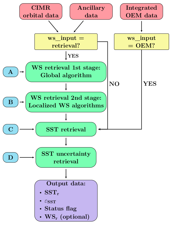
Fig. 1 Set-up of the PMW SST retrieval algorithm using CIMR orbital data and ancillary data as input. \(\boldsymbol{\mathrm{A}}\), \(\boldsymbol{\mathrm{B}}\), \(\boldsymbol{\mathrm{C}}\) and \(\boldsymbol{\mathrm{D}}\) refer to the regression coefficients in Equations (1), (4), (6) and (8), respectively.#
Retrieval algorithm#
The retrieval algorithm is a statistically-based algorithm for retrieving SST given satellite TBs and ancillary data, such as e.g. WS. The main option is to use retrieved WS from the integrated OEM retrieval. Two additional options exist; the use of ancillary WS, from e.g. reanalysis data, or retrieval of WS using a 2-stage WS retrieval algorithm.
Mathematical description#
WS retrieval algorithm#
Optionally, a statistical retrieval algorithm can be used to retrieve WS given satellite TBs and ancillary data. The WS retrieval algorithm is a two-stage algorithm based on the multiple linear regression model from Alerskans et al. [2020]. In the first stage, an initial estimate of WS is retrieved using a so called global regression-based retrieval algorithm, i.e. the model uses one set of regression coefficient for all retrievals. In the second stage, a final estimate of WS is obtained through the use of localized algorithms, such that different sets of regression coefficients are used for the retrievals. Here, the retrieved WS from the 1st-stage retrieveq_sst_uncertal is used to bin the data and regression coefficients are obtained for a set of pre-defined WS intervals. Hence, the 2nd-stage retrieval algorithm is trained to perform well over restricted WS domains.
1st-stage: Global retrieval algorithm#
The first stage of the WS retrieval algorithm uses a global regression model to obtain regression coefficients based on all training examples in the training dataset. The WS retrieval algorithm is based on the NOAA AMSR2 WS retrieval algorithm [Chang et al., 2015] and uses TBs and Earth incidence angle (\(\theta_{EIA}\)) to obtain initial retrieved WS, \(WS_a\),
where
and
The summation index \(i\) represents the summation over the \(N_{ch}=8\) channels included in the retrieval algorithm: 6.9, 10.6, 18.7, and 36.5 (dual polarizations), and the coefficients \(a_0\) to \(a_3\) are the regression coefficients, here together referred to as \(A\), determined using the least-squares method.
2nd-stage: WS loclised retrieval algorithm#
Localized WS retrieval algorithms are used in the second stage of the WS retrieval algorithm. Here, the algorithms are defined for local WS bins, such that separate regression coefficients are derived for each WS interval, where \(WS_{a}\) is used to select the correct WS bin. In order to obtain robust regression coefficients, the minimum number of matchups required were set to 100. The localized algorithms are defined for WS in the interval 0 to 20 ms\(^{-1}\), with a bin size of 1 ms\(^{-1}\), which gives a total of 20 localized algorithms. Like the 1st-stage retrieval, TB and incidence angle are used in the localized WS algorithm to obtain a final estimate of WS, \(WS_r\),
where \(t_{i}\) is given by Equation (2) and \(\theta\) is defined by Equation (3). The index \(i\) refers to the summation over all \(N_{ch}\) channels included in the retrieval algorithm, \(k\) refers to the reference WS bin and the coefficients \(b_{0}\) to \(b_{3}\) are regression coefficients, here together referred to as \(B\), determined using the least-squares method. The final retrieved WS is found by performing a linear interpolation between \(WS_{rk}\) and the WS retrieved using the closest neighboring WS algorithm in order to avoid discontinuities
where the interpolation weights \(w\) are given by \(w_{0}=1-\alpha\) and \(w_{1}=\alpha\), with \(\alpha=\frac{WS_{\alpha}}{\Delta k}-k_{0}\) and \(k_{0}=floor(\frac{WS_{r}}{\Delta k})\), where \(\Delta k=1~ms^{-1}\) is the WS bin size.
SST retrieval algorithm#
A statistical retrieval algorithm is used to retrieve SST given satellite TBs and ancillary data. The SST retrieval algorithm is based on multiple linear regression and uses a global regression model to obtain regression coefficients based on all training examples in the training dataset. The algorithm is inspired by the RSS AMSR-E SST retrieval algorithm [Wentz and Meissner, 2000] and the retrieval algorithm from Alerskans et al. [2020], in which the SST is retrieved using TBs, Earth incidence angle, retrieved WS and the relative angle between wind direction and satellite azimuth angle (\(\phi_{rel}\))
where again \(t_{i}\) is given by Equation (2) and \(\theta\) is defined by Equation (3). The index \(i\) refers to the summation over all \(N_{ch}\) channels included in the retrieval algorithm; 6.9, 10.6, 18.7 and 36.5 GHz (dual polarization), and the coefficients \(c_{0}\) to \(c_{6}\) are regression coefficients, here together referred to as \(C\), determined using the least-squares method.
SST uncertainty retrieval algorithm#
Following the approach used within the ESACCI SST project, the total uncertainty of the retrieved SST, \(\varepsilon_{SST}\) is a combination of three uncertainty components; a random uncertainty component, \(\varepsilon_{rand}\), a local systematic uncertainty component, \(\varepsilon_{local}\), and a global systematic uncertainty component, \(\varepsilon_{global}\)
The local systematic and the random uncertainty components are obtained through the use of a regression model, based on the algorithm developed and applied in Alerskans et al. [2020]. The algorithm uses retrieved SST, (retrieved) WS, solar zenith angle (\(\theta_{sza}\)) and latitude (\(\varphi_{lat}\))
where the coefficients \(d_0\) to \(d_8\) are regression coefficients, here together referred to as \(D\), determined using the least-squares method. One set of regression coefficients are obtained for the random uncertainty component and another set of coefficients are obtained for the local systematic uncertainty component. The global uncertainty component, however, is assumed to be small and therefore set to zero, following Alerskans et al. [2020].
The random uncertainty component is related to the NEdT and therefore, to estimate it the NEdT of the TBs is propagated through the SST retrieval algorithm to obtain a new set of SSTs, called \(SST_{r,rnd}\). In order to obtain the regression coefficients, a pre-binning of the training data is performed for SST, WS, solar zenith angle and latitude according to Table 2. Based on this, two standard deviation estimates are computed; (i) \(\sigma_{\Delta SST_r}\), which is the standard deviation of \(SST_r\) minus the in situ SST and is used to represent local effects and also includes the in situ uncertainty and sampling effects, and (ii) \(\sigma_{\Delta SST_{r,rnd}}\), which is the standard deviation of \(SST_r\) minus \(SST_{r,rnd}\) and is used to represent random effects. The regression coefficients for the random uncertainty component are obtained through training of the algorithm against \(\sigma_{\Delta SST_{r,rnd}}\), whereas the corresponding regression coefficients for the local systematic uncertainty component are obtained through training against local variations in \(\sigma_{\Delta SST_r}\) only.
variable |
bin size |
min |
max |
|---|---|---|---|
SST |
\(2^{\circ}\)C |
\(-1^{\circ}\)C |
\(33^{\circ}\)C |
WS |
\(2\) ms\(^{-1}\) |
\(-1\) ms\(^{-1}\) |
\(33\) ms\(^{-1}\) |
\(\varphi_{lat}\) |
\(10^{\circ}\) |
\(-85^{\circ}\) |
\(85^{\circ}\) |
\(\theta_{sza}\) |
\(15^{\circ}\) |
\(7.5^{\circ}\) |
\(172.5^{\circ}\) |
Status flag#
The retrieved SSTs are each assigned a status flag according to Table 3 to indicate the quality of the individual retrievals.
level |
definition |
|---|---|
0 |
no data |
1 |
bad data |
2 |
worst-quality usable data |
3 |
low quality data |
4 |
acceptable quality data |
5 |
best quality data |
Input data#
In the initial phase, the ESA CCI MMD will be used for algorithm development and tuning. The ESA CCI MMD, previously described in Nielsen-Englyst et al. [2018] and Alerskans et al. [2020], contains TBs from the AMSR-E level 2A and AMSR2 level 1R swath data products [Ashcroft and Wentz, 2013, Maeda et al., 2016]. It also includes quality controlled in situ SST observations from the International Comprehensive Ocean-Atmosphere DataSet version 2.5.1 [Woodruff et al., 2011] and the Met Office Hadley Centre Ensembles dataset version 4.2.0 [Good et al., 2013]. Additional data include reanalysis data from the ERA-Interim [Dee et al., 2011] and ERA5 reanalyses [Hersbach et al., 2020]. The MMD includes temporally matched and collocated matchups from the period June 2002 - October 2011 and July 2012 - December 2016.
AMSR2 TBs will be used for the initial algorithm development and validation. A CIMR-like channel combination will be used, based on Nielsen-Englyst et al. [2021]. For this set-up, necessary PMW observations are:
Furthermore, the use of simulated CIMR TBs in the development of the algorithm will be investigated. This has the advantage of including the L-band TBs, which are not available from AMSR2.
The next phase will see the use of CIMR orbital data and here the following input data are needed:
Output data#
The outputs from the regression retrieval algorithm are:
Sea surface temperature (\(SST_{r}\)), in Kelvin
Sea surface temperature uncertainty (\(\varepsilon_{SST}\)), in Kelvin
Status flag
Wind speed (\(WS_{r}\)), in ms\(^{-1}\) (optional)
Auxiliary data#
Data that is used as a complement to the retrieval, such as for flagging:
Sea ice product
Distance to coast
Sun glint information
Information for RFI flagging
Ancillary data#
Data necessary for the retrieval:
Earth incidence angle (satellite zenith angle)
Satellite azimuth angle
Reanalysis surface winds
Validation process#
Validation of the Level-2 SST product is based on comparison of retrieved SST with collocated and temporally matched in situ observations. In the initial phase, the ESA CCI MMD is used for evaluation of the CIMR SST algorithm performance. The metrics used for the validation are standard verification metrics such as bias, standard deviation, root mean square error (RMSE) and coefficient of correlation.
Furthermore, the validation process will also include validation on Picasso scenes.