Algorithm Performance Assessment

This chapter presents a performance assessment of the prototype soil moisture retrieval algorithm based on end-to-end simulations of a synthetic reference scenario.

Reference Scenario definition

A synthetic soil moisture test card was created to serve as a testbed for the soil moisture retrieval algorithm.

The test card has a spatial resolution of 1 km, which is nested within the global 9 km and 36 km EASE2 grids. At L-, C-, and X-bands, the brightness temperature signatures are based on numerical simulations of a discrete radiative transfer model (Tor Vergata model) [Ferrazzoli et al., 2002, Guerriero et al., 2016]. At Ku- and Ka-bands, brightness temperature signatures are based on forward simulations of the tau-omega model (not used in this prototype) [Mo et al., 1982]. Five land use classes are considered: Bare soil, grassland, cropland, mixed, and forest. The mixed class assumes an homogeneous mix of grassland, cropland, and forest.

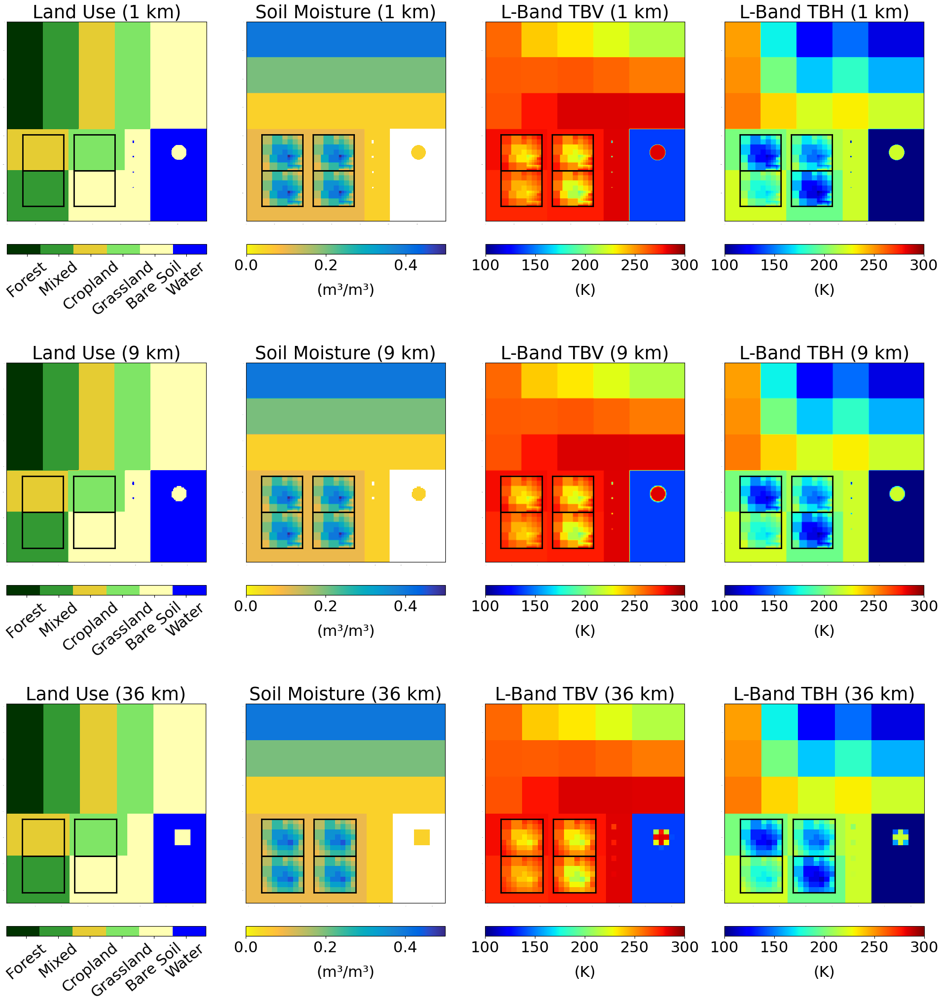
Fig. 5 Synthetic soil moisture test card at 1 km (top, native resolution), 9 km (middle, aggregated) and 36 km (bottom, aggregated). Columns indicate the dominant land use, average soil moisture content, and L-band brightness temperatures at V- and H-polarization, respectively. Brightness temperatures at C-, X-, Ku-, Ka-bands are not shown for brevity.

Fig. 5 shows the synthetic test card for 1 km (native resolution), 9 km, and 36 km resolutions. The soil moisture fields at 9 km and 36 km resolutions will be used as a reference for the performance evaluation. Four areas of interest (AOIs) are indicated by black boxes. These areas indicate four distinct land use classes that contain identical soil moisture patterns.

Performance Metrics

Two algorithm performance metrics are used in the evaluation: The unbiased root mean squared error (ubRMSE) and the bias of soil moisture retrievals with respect to the synthetic reference. These metrics correspond to standard performance metrics for soil moisture retrievals [Entekhabi et al., 2010].

We test the prototype algorithm on four simulated L1B files, which represent distinct CIMR overpasses. The L1B files are based on orbit simulations conducted by DEIMOS and the SCEPS project. Each orbit simulator covers one ascending and descending orbit, respectively.

Prototype Algorithm Results

Regridding

The purpose of regridding is to move from L1B TBs, provided in swath geometry, to gridded TBs, posted on a global EASE2 grid. In a first step, we grid L-band TBs to the 36 km global EASE2 grid, using a Gaussian regridding. We also grid C-band TBs to the 9 km grid using the same technique (Note: More advanced gridding techniques, such as the Backus-Gilbert optimal interpolation technique, are planned to be implemented in a separate toolbox).

In a second step, we sharpen the L-band TBs by means of the following procedure, which takes lower-resolution L-band TBs (36 km grid) and higher-resolution C-band TBs (9 km grid) as inputs:

\[ TB_L(9 km) = \frac{TB_L(36 km)}{TB_C(36 km)} TB_C(9 km), \]

where \(TB_C(36 km)\) is the aggregation of \(TB_C(9 km)\) to the 36 km grid. The procedure is similar to the smoothing filter-based intensity modulation technique (SFIM) [Santi, 2010], while preserving the mean L-band TB of each 36 km pixel. The final sharpening algorithm for CIMR will be determined based on further tests. Should C-band TBs be affected by radio frequency interference, the same technique can also be applied using X-band TBs, leading to comparable results (not shown).

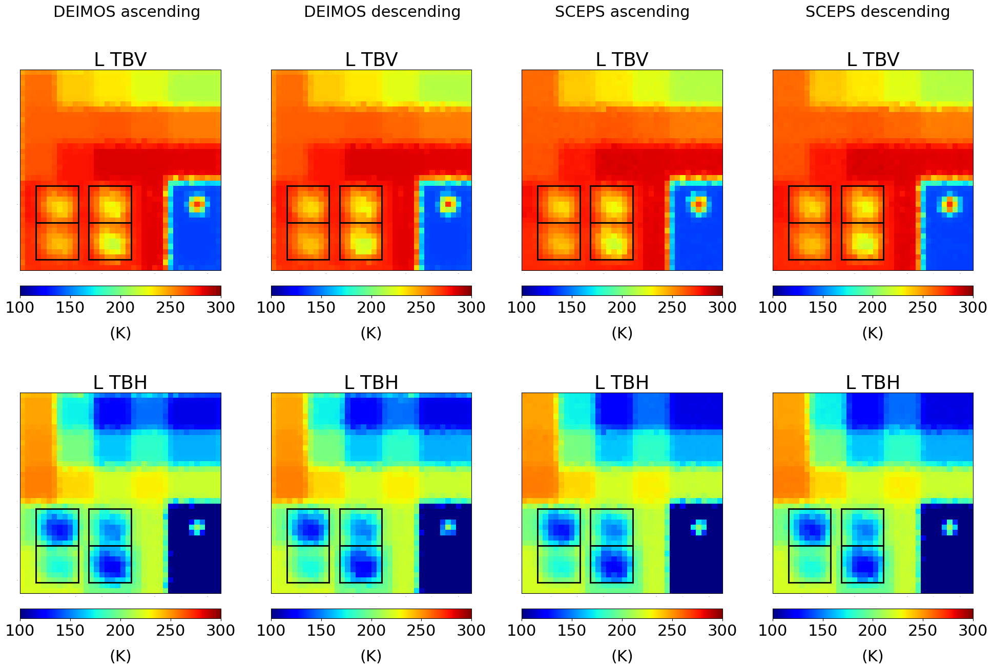
Fig. 6 L-band brightness temperature signatures posted on a 36 km global EASE2 grid.

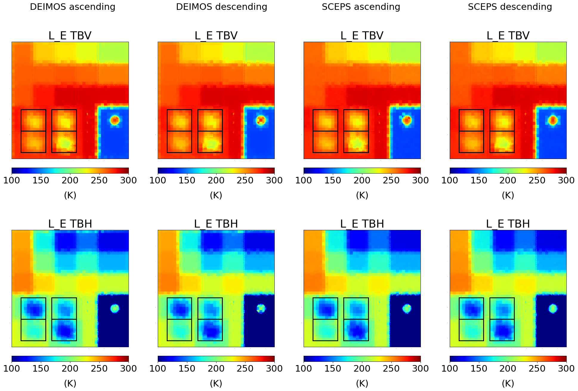
Fig. 7 L-band brightness temperature signatures (sharpened with C-band) posted on a 9 km global EASE2 grid.

Soil Moisture Retrieval

We apply the prototype soil moisture retrieval algorithm to the gridded L-band TBs. The results for the 36 km and 9 km grids are shown in Fig. 8 and Fig. 9, respectively. We also show outputs for vegetation optical depth (VOD), noting that VOD is not a target variable of the algorithm and will not be part of the performance evaluation.

We find that soil moisture patterns are captured well across all land use types. VOD retrievals correspond to expected patterns of different land use classes, noting that cropland and grassland are almost transparent at L-band for the test card scenario considered here. A more detailed assessment of the results is given in the next section.

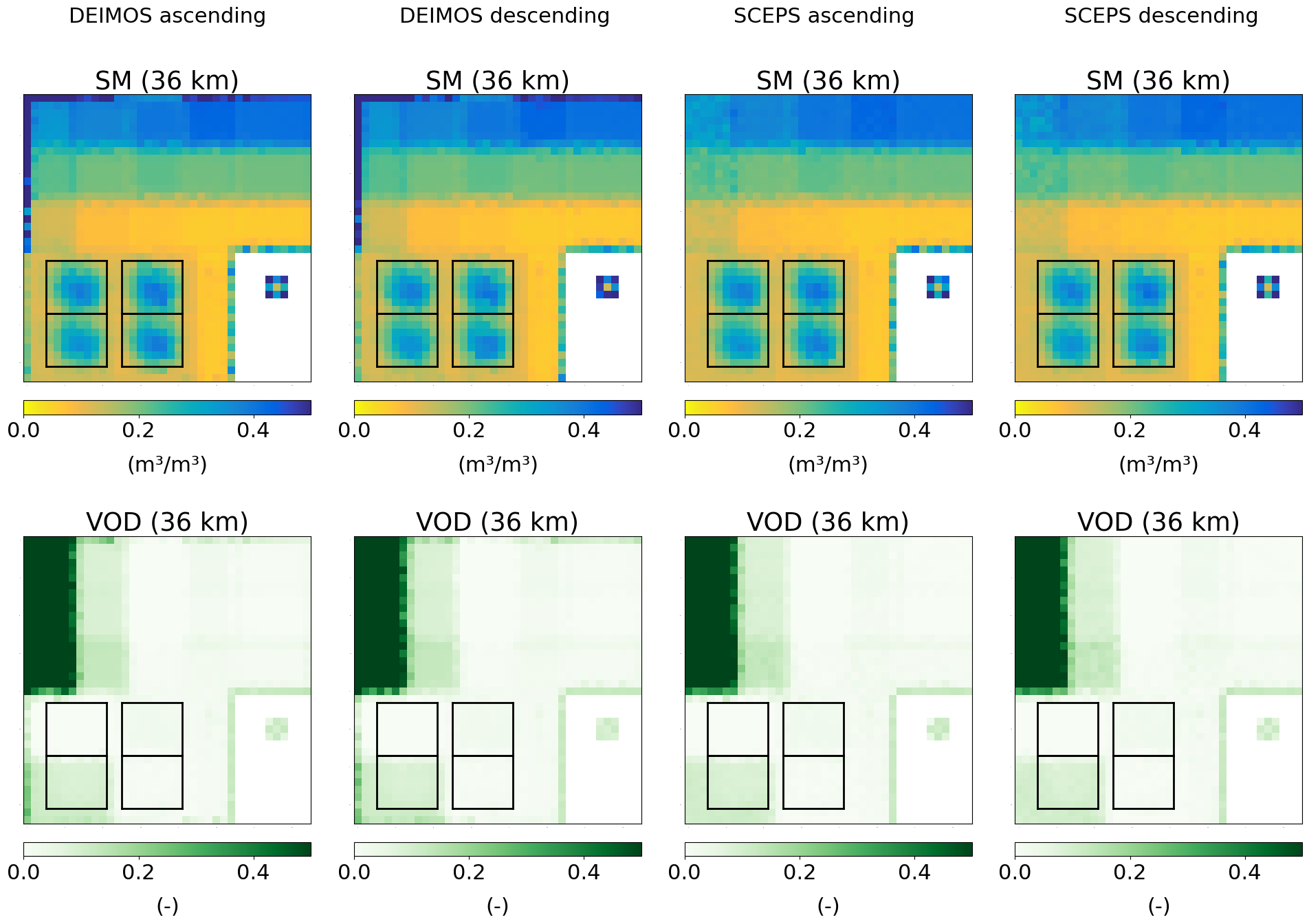
Fig. 8 Soil moisture and vegetation optical depth (VOD) retrieval results of the prototype algorithm at the 36 km resolution.

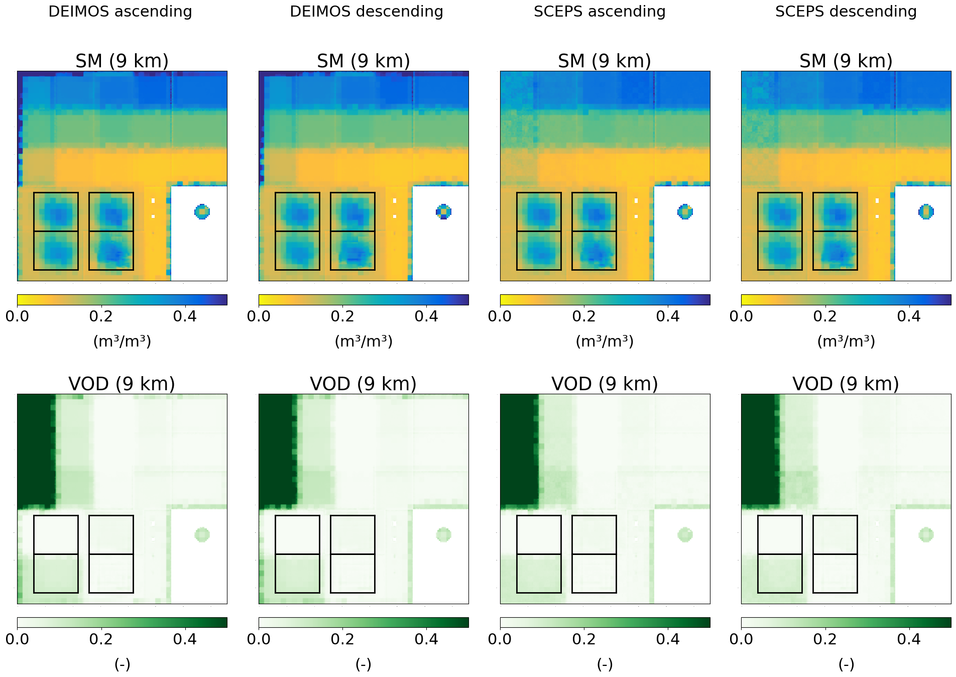
Fig. 9 Soil moisture and vegetation optical depth (VOD) retrieval results of the prototype algorithm at the 9 km resolution.

Algorithm Performance Assessment

We evaluate the prototype algorithm retrievals against the synthetic reference in Fig. 10 and Fig. 11.

We find that the soil moisture fields are generally in good agreement with the synthetic reference in Fig. 5. The soil moisture patterns in the AOIs (black boxes) are well captured, indicating that soil moisture retrievals are consistent across different spatial scales and land use classes. Soil moisture retrievals within the AOIs show no systematic biases across the soil moisture range, with the exception of the mixed land use class (bottom left), which shows a dry bias for wet soil moisture conditions. Biases in the AOIs are further discussed in Fig. 13 and Fig. 14.

Several observations apply to explain the error patterns throughout the test card. The largest errors occur near the coastlines, which is expected due to spillover effects from ocean TBs. A land-water correction of TBs is planned for CIMR but is not applied in this study. Large errors also occur at the edge of the DEIMOS scenes, which is a spillover effect from the background field used in the L1B simulations. A slight wet bias is visible for bare soil areas, which represent very dry soil conditions. These areas serve to depict a strong TB contrast between dry soil and the adjacent ocean. It is expected that these biases could be reduced by calibrating the roughness parameters, which is deliberately not conducted for the synthetic dataset assessed here. Notable biases occur also for forest regions, which is expected due to the heavy masking of the soil signal by the dense vegetation. The two SCEPS scenes show effects of instrument noise particularly for forest retrievals (instrument noise is not considered in the DEIMOS scenes), which is attributed to the same effect. Overall, barring minor differences across orbit simulators, the prototype algorithm captures soil moisture patterns consistently across land use classes and overpasses.

Two additional observations apply to 9 km retrievals in Fig. 11: First, vertical edge effects are visible in the northeastern corner of the test card, which is an artifact resulting from the sharp land cover transitions in the synthetic test card. Second, additional error patterns are visible within the AOIs compared to 36 km retrievals, which is expected from the higher resolution of the synthetic reference. A more detailed view of the 9 km retrievals in the AOIs is given in Fig. 12.

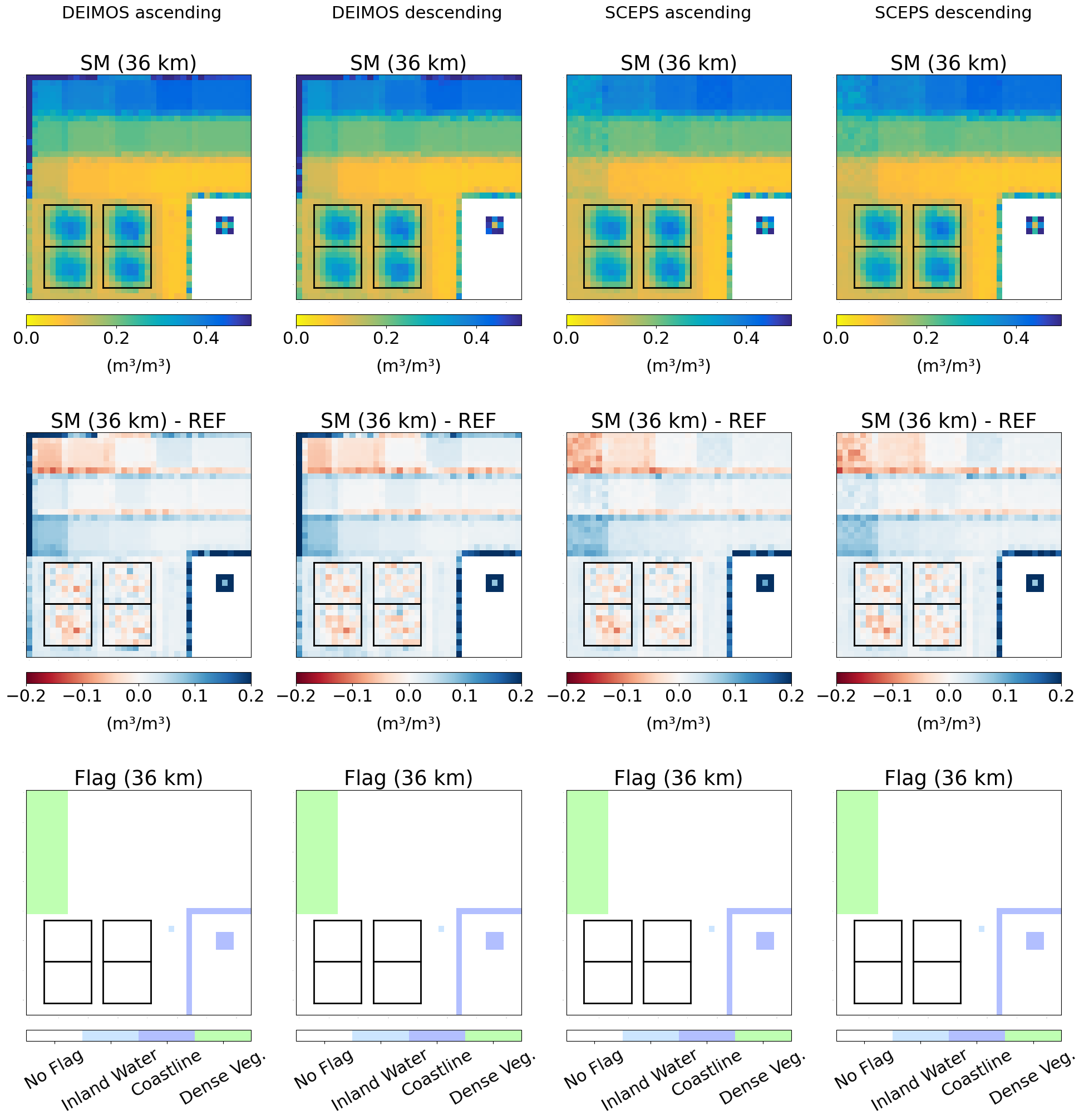
Fig. 10 Soil moisture retrieval results of the prototype algorithm at the 36 km resolution (top row). Difference with respect to the synthetic reference, aggregated to the same resolution (middle row). Retrieval scene flags that indicate uncertain retrievals (bottom row).

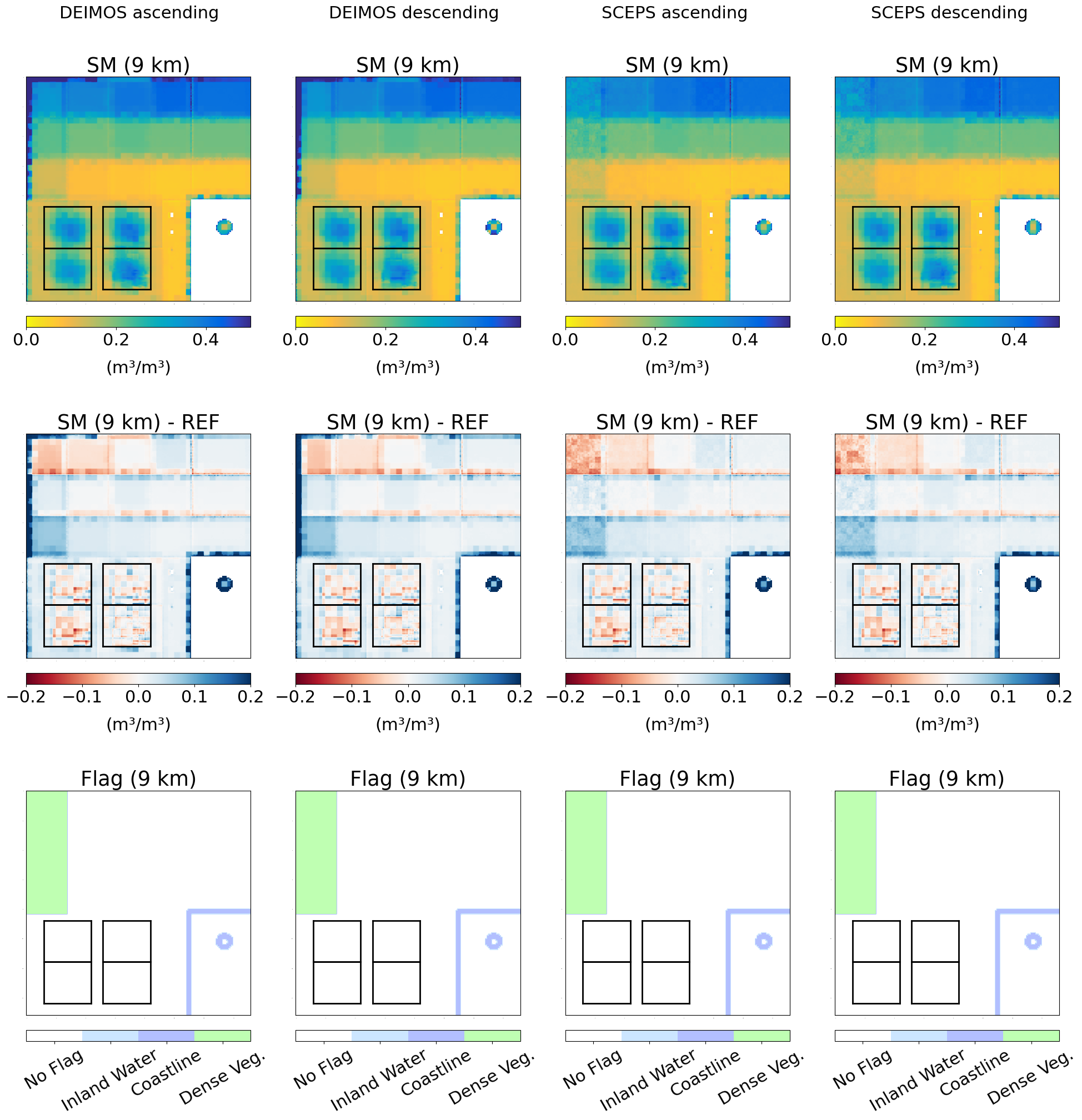
Fig. 11 Soil moisture retrieval results of the prototype algorithm at the 9 km resolution (top row). Difference with respect to the synthetic reference, aggregated to the same resolution (middle row). Retrieval scene flags that indicate uncertain retrievals (bottom row).

Fig. 12 shows a more detailed view of the 36 km and 9 km retrievals in the AOIs.

At the 36 km grid, soil moisture patterns are reasonably captured by the retrievals. Note that the retrievals do not capture the full spatial dynamic range of the reference in all cases (i.e., the wettest pixel is not fully resolved), which is expected as the L-band footprint of CIMR is significantly larger than the 36 km grid, and a simple Gaussian regridding was applied in this prototype implementation. By exploiting the oversampling of CIMR, it is expected that more advanced regridding techniques can further improve the capabilities to capture spatial patterns at the 36 km scale. For the mixed land use class (bottom left AOI), soil moisture retrievals show a dry bias for wet soil moisture conditions, as was mentioned earlier. This is likely related to vegetation masking of the soil signal, which further reduces the dynamic range of the observed TBs.

At the 9 km grid, the high resolution reference soil moisture patterns are captured particularly well for bare soil (bottom right AOI) and grassland (top right AOI). This is expected as the C-band signal from the soil gets increasingly masked with increasing vegetation cover. Biases in the 36 km retrievals carry over to the sharpened 9 km retrievals, such that the dry bias for the mixed class is also observed here. Note that the synthetic test card assessed here does not show spatial land cover variability at the 9 km scale, which limits the available brightness temperature variability to be captured by the sharpening algorithm. It is expected that the added value of the sharpening would increase further for scenes that include spatial land cover heterogeneity, particularly for land use classes with increased vegetation cover. The results are based on sharpening of L-band TBs with C-band TBs. Comparable results are obtained for X-band TBs (not shown).

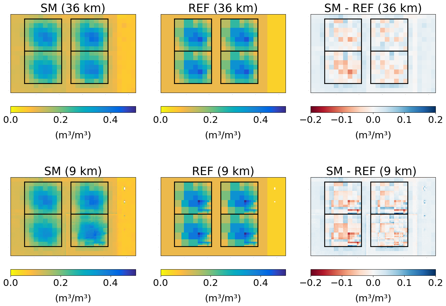
Fig. 12 Comparison of 36 km (top row) and 9 km (bottom row) retrievals. AOIs in black boxes depict bare soil, grassland, cropland, and mixed land use (counterclockwise, from the bottom right).

Finally, ubRMSE and bias metrics are displayed in Fig. 13 and Fig. 14, respectively. We assess four land use classes: Bare soil, grassland, cropland, and mixed. These classes correspond to vegetation water contents (VWC) of 0 kg/m², 0.2 kg/m², 1.9 kg/m², 4.6 kg/m², respectively. Forest regions show a vegetation water content of 11.7 kg/m² and are not considered in the evaluation. The metrics are calculated for AOIs containing identical soil moisture patterns, which are indicated as black boxes in Fig. 8 to Fig. 12.

We find that the prototype algorithm achieves an ubRMSE smaller than 0.04 m³/m³ for 36 km retrievals and between 0.035 - 0.045 m³/m³ for 9 km retrievals. Errors generally increase with increasing vegetation cover, in accordance with expectations. Biases are overall low. The largest biases, occurring in the mixed class, do not exceed 0.01 m³/m³. For all classes, the ubRMSE and bias metrics show a high level of consistency across overpasses.

Note that the performance assessment metrics are achieved without parameter calibration: The soil roughness (H) and single scattering albedo (⍵) parameters follow strictly the values proposed in Table 3 and are not calibrated to provide an optimal fit for the simulated brightness temperature signatures (Note that the ⍵ parameter was adjusted for forest retrievals to enable retrievals despite the excessive vegetation cover. Forest retrievals are not part of the performance metrics calculation). It is expected that the performance metrics could be further improved if the algorithm parameters were specifically tuned to the synthetic TB simulations.

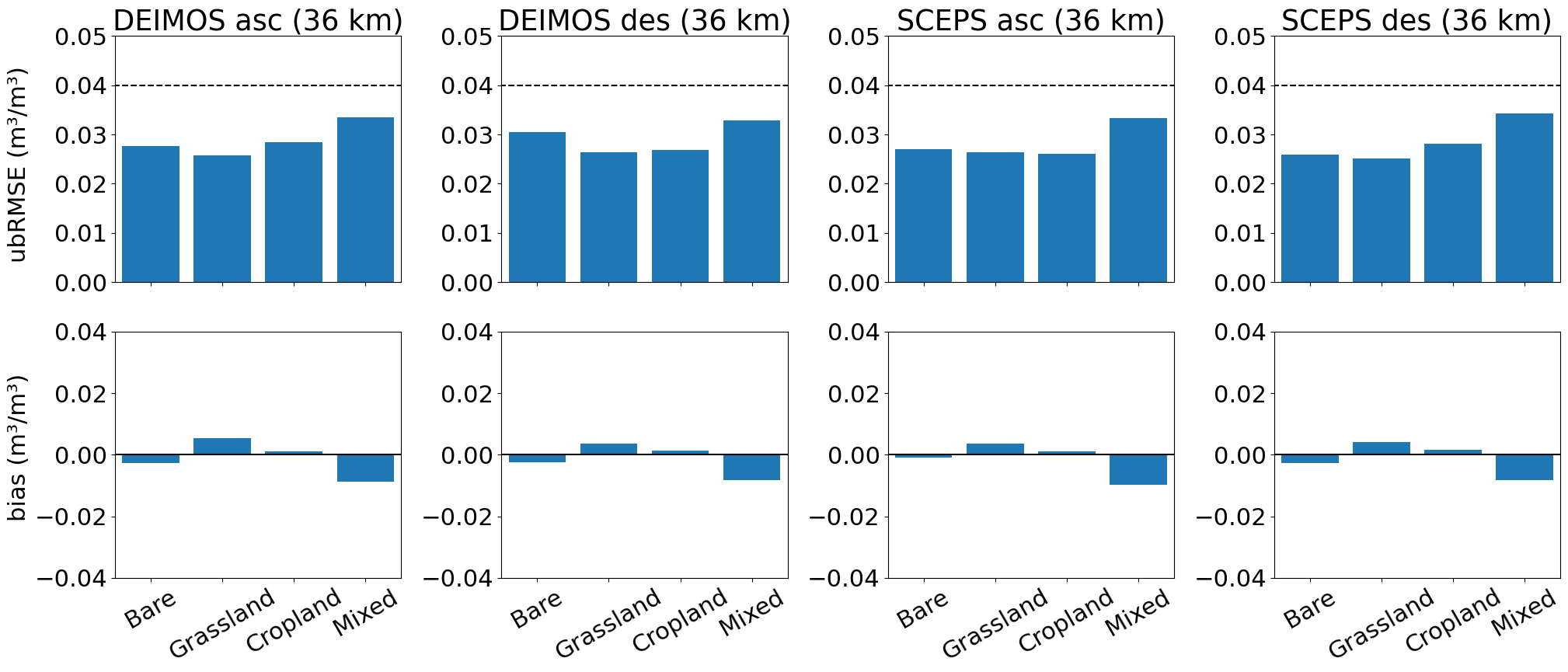
Fig. 13 ubRMSE and bias metrics for soil moisture retrievals at the 36 km scale.

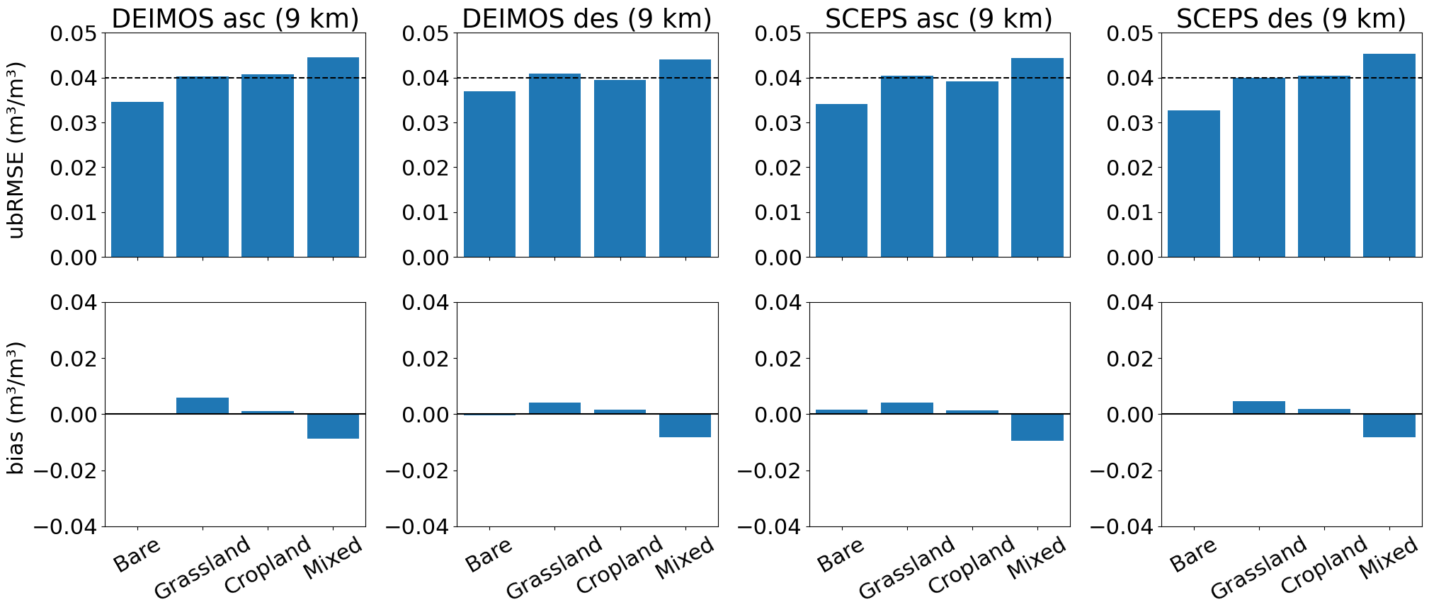
Fig. 14 ubRMSE and bias metrics for soil moisture retrievals at the 9 km scale.

Overall, the results provide a promising outlook on the prototype SM retrieval algorithm for CIMR.

The key results for the AOIs, which are the target of the assessment, are summarized below:

• At the 36 km scale, the algorithm shows an ubRMSE < 0.04 m³/m³.

• At the 9 km scale, the algorithm shows an ubRMSE between 0.035 - 0.045 m³/m³.

• Biases are overall low and do not exceed 0.01 m³/m³.

• The results are consistent across overpasses.

• All metrics are achieved without parameter calibration.

Acknowledgements

Paolo Ferrazzoli and Leila Guerriero are acknowledged for providing the code of the Tor Vergata model and helpful discussions on the forward simulations.