Baseline Algorithm Definition

Extensive research in the passive microwave soil moisture field has led to the development of numerous soil moisture retrievals that can be applied to CIMR TB data. The ESA’s SMOS mission currently operates an aperture synthesis L-band radiometer that produces TB data at various incidence angles for identical ground locations. The core SMOS retrieval algorithm utilizes the tau-omega model and takes advantage of SMOS’s ability to capture multiple incidence angles for soil moisture estimation. SMAP retrievals, on the other hand, are also based on the tau-omega model but employ the constant incidence angle TB data provided by the SMAP radiometer, an approach more similar to the forthcoming CIMR mission. Consequently, we propose a retrieval algorithm that incorporates elements from both the SMOS-IC and SMAP dual-channel algorithms.

A microwave radiometer’s primary function is to detect the inherent thermal radiation that originates from a surface. The brightness temperature (TB) measured by a radiometer is proportional to the product of the surface’s temperature and emissivity.

When the microwave sensor orbits the Earth, several factors contribute to the observed TB. These include the soil’s emitted energy (attenuated by overlying vegetation), the emission from vegetation itself, downwelling atmospheric emission and cosmic background emission (reflected by the surface and attenuated by vegetation), and upwelling atmospheric emission.

In the case of L-band frequencies, the atmosphere is close to transparent, with an atmospheric transmissivity (\(τ_{atm}\)) of approximately 1. The cosmic background, or \(T_{sky}\), is around 2.7 K. Additionally, atmospheric emission is minimal.

Forward Model

The retrieval of soil moisture and microwave vegetation parameters from CIMR surface TB observations relies on a widely recognized zeroth-order solution to the radiative transfer equation referred to as the tau-omega model [Mo et al., 1982], which, in this document, is referred to as the forward model. In tau-omega, the total upwelling emission is composed of a soil contribution, a vegetation contribution and a soil-scattered vegetation contribution. It assumes a weakly scattering medium (e.g. no multiple scattering). \(τ\) is the vegetation optical depth (VOD) that quantifies the total attenuation within the canopy, while \(ω\) is the vegetation single scattering albedo, i.e., the ratio of scattering to extinction, ranging from zero to one ([Mo et al., 1982];[Ulaby and Long, 2014]). The tau-omega model is formulated as:

(1)\[TB_p = T_s e_p \exp{(-\tau \sec \theta)} + T_c (1 - \omega)[1 - \exp(-\tau \sec \theta)][1 + r_p \exp(-\tau \sec \theta)]\]

Where the subscript p refers to polarization (V or H), \(T_s\) denotes the soil temperature and \(T_c\) stands for the canopy temperature, and \(r_p\) is the soil reflectivity of a rough surface. The reflectivity is connected to the emissivity (\(e_p\)) through the relation \(e_p = (1 - r_p)\). Note that \(τ\) and \(ω\) are theoretically polarization dependent, but are assumed to be polarization independent across satellite-scale retrieval applications ([Wigneron et al., 2007]). It must be noted that \(\omega\) will be treated here as an effective parameter [Kurum, 2013].

According to Beer’s law, the overlying canopy layer’s transmissivity or vegetation attenuation factor , \(\gamma\), is given by \(\gamma = \exp(-𝜏 \sec \theta)\). Equation (1) assumes that vegetation multiple scattering and reflection at the vegetation-air interface are negligible.

Surface roughness is modeled as \(r_p = r^*_p \exp(-H_R \cos^n(\theta))\), where \(H_R\) and \(n\) parameterize the intensity of the roughness effects, and \(r^*_p\) stands for the reflectivity of a plane surface [Wang and Choudhury, 1981, Lawrence et al., 2013]. The surface reflectance \(r^*_p\) is characterized by the Fresnel equations, which detail the actions of an electromagnetic wave when interacting with a smooth surface. When an electromagnetic wave encounters a surface that separates two media with different dielectric properties (e.g., air and soil), part of the wave’s energy is reflected at the surface, and part is transmitted through it. The Fresnel equations are used to calculate the amount of energy reflected based on the incident angle of the wave and the dielectric properties of the involved media. For horizontal polarization, the wave’s electric field aligns parallel to the reflecting surface and perpendicular to the propagation direction. In contrast, for vertical polarization, the electric field of the wave has a component perpendicular to the surface. Equations (2) and (3) show the Fresnel equations for horizontal and vertical polarizations, respectively.

(2)\[r^*_H(\theta) = \left| \frac{\cos\theta - \sqrt{\epsilon - \sin^2\theta}}{\cos\theta + \sqrt{\epsilon - \sin^2\theta}} \right|^2\]

(3)\[r^*_V(\theta) = \left| \frac{\epsilon\cos\theta - \sqrt{\epsilon - \sin^2\theta}}{\epsilon\cos\theta + \sqrt{\epsilon - \sin^2\theta}} \right|^2\]

where \(\theta\) represents the CIMR incidence angle, while \(\epsilon\) denotes the soil layer’s complex dielectric constant.

It is important to note that an increase in soil moisture is accompanied by a proportional increase in the soil dielectric constant (\(\epsilon\)). For instance, liquid water has a dielectric constant of 80, while dry soil possesses a dielectric constant of 5. Furthermore, it should be acknowledged that a low dielectric constant is not uniquely indicative of dry soil conditions. Frozen soil, regardless of water content, exhibits a dielectric constant similar to that of dry soil. Consequently, a freeze/thaw flag is required to resolve this ambiguity. Since TB is proportional to emissivity for a given surface soil temperature, TB decreases as soil moisture increases. In the CIMR algorithm, \(\epsilon\) is expressed as a function of SM, soil clay fraction and soil temperature using the model developed by Mironov [Mironov et al., 2012].

This relationship between soil moisture and soil dielectric constant (and consequently microwave emissivity and brightness temperature) establishes the basis for passive remote sensing of soil moisture. With CIMR observations of TB and auxiliary information on \(T_s\), \(T_c\), \(H_R\), and \(\omega\), soil moisture (SM) and vegetation optical depth (VOD) can be retrieved.

Retrieval Method

Prior to implementing the soil moisture retrieval, a preliminary step is to perform a water body correction to the brightness temperature data for cases where a significant percentage of the grid cells contain open water. As it is well known, brightness temperature values notably decrease when the water fraction increases [Ulaby and Long, 2014], leading to an overestimation of the retrieved SM values [Ye et al., 2015] and inducing artificial seasonal cycles of VOD [Bousquet et al., 2021]. It is therefore important to correct the CIMR brightness temperatures for the presence of water, to the extent feasible, prior to using them as inputs to the Level-2 Soil Moisture retrieval. This correction needs to be performed using the CIMR Hydrology Target mask ([RD-1] MRD-854), as part of the optimal interpolation or re-sampling process (in the CIMR RGB toolbox). The hydrology target mask will include information from both permanent and transitory water surfaces that shall be identified with the surface water seasonality information provided by the CIMR Surface Water Fraction (SWF) product as well as ancillary information.

The procedure to acquire soil moisture (SM) and vegetation optical depth (VOD, also denoted as \(\tau\)) from L-band TBs requires the minimization of the cost function F, as shown in (4):

(4)\[F(SM, \tau) = \displaystyle \sum_{p=h,v} \frac{(TB_p^{obs} - TB_p^{mod})^2}{\sigma_{TB}^2} + \frac{(\tau^{ini} - \tau)^2}{\sigma_\tau^2}\]

where the term \(TB_p^\text{obs}\) refers to the observed brightness temperature, \(\sigma_{TB}\) denotes the standard deviation associated with the brightness temperature measurements (a constant value of 1 K is initially proposed), and \(TB_p^{mod}\) is the brightness temperature calculated using (1). The cost function also incorporates a regularization term, where \(\tau\) represents the retrieved VOD, \(\tau^\text{ini}\) is an a priori estimate calculated from previous runs, and \(\sigma_\tau\) is its associated standard deviation. A regularization term for SM, which is employed in SMOS-IC, is not currently included. The exact regularization strategy, including the weights of the cost function terms (goverend by \(\sigma_{TB}\) and \(\sigma_\tau\)), will be determined based on further tests. The current optimization method is the Trust Region Reflective algorithm [Branch et al., 1999].

Prior to retrieval of SM, ancillary data will be employed to help to determine whether masks are in effect for strong topography, urban, snow/ice, frozen soil.

CIMR Level-1b re-sampling approach

The CIMR Level-2 Soil Moisture retrieval algorithm will provide two soil moisture products: the first based on the inversion of L-band only TBs at its native resolution (<60 km, Hydroclimatological), the second one based on the inversion of L-band at an enhanced spatial resolution (~10 to 25 km Hydrometeorological). The enhanced L-band targets an effective mean spatial resolution of 15 km and is based on sharpening techniques that exploit the C-band and X-band channels ([Santi, 2010], [Santi et al., 2018], [Zhang et al., 2025]).

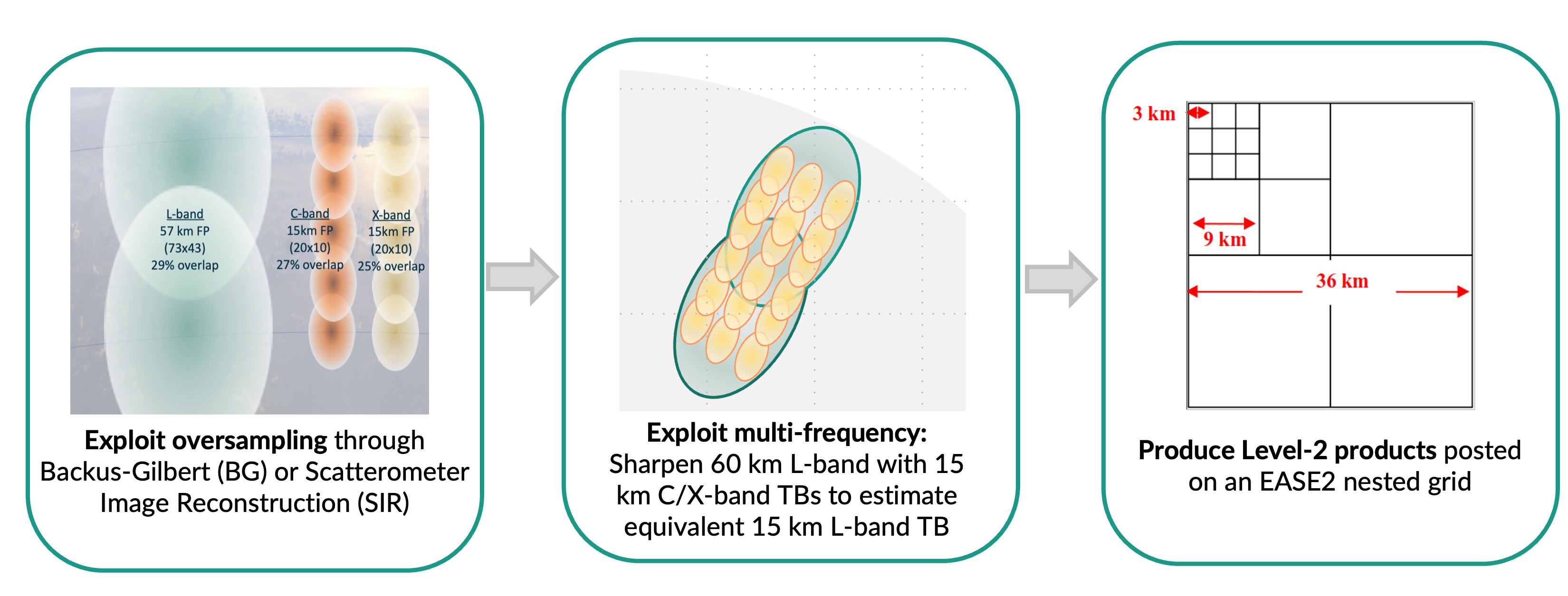
Fig. 3 Conceptual flow of Level-1B resampling to exploit CIMR oversampling, multifrequency and nested spatial resolution to meet soil moisture observational requirements.

The CIMR Level-1b re-sampling and re-mapping approach is illustrated in Fig. 3. In a first step, the Level-1b TBs will be remapped on common location using a Backus-Gilbert or Scatterometer Image Reconstruction techniques (in a separate CIMR RGB Toolbox). The objective of this first step is to optimize L-band reconstruction to provide the highest possible spatial resolution at the lowest noise level [Long et al., 2019] (TB_L product). In a second step, which is exclusive to the TB_L_E product, an sharpening algorithm will be applied to combine lower resolution L-band TBs with higher resolution C-/X-band TBs to provide an equivalent estimate of high resolution L-band TBs. Both the TB_L and TB_L_E products will be posted on global EASE2 grids with a kernel of 3 km (then multiples thereof). The effective spatial resolution of both products, targeted to be <60 km (L-band only) and ~15 km (after sharpening using C/X bands), will be evaluated and compared (e.g. as in [Long et al., 2023]). The CIMR radiometer is conically scanning and its high degree of oversampling provides flexibility in resampling the data, supporting the use of a finer grid (posting resolution) than the TB effective resolution [Long et al., 2023]. At L-band, CIMR TB measurements are collected with an along-scan spacing of approximately 8 km, while there is an overlap of 29 % in the along-track direction (no spacing). In order to preserve as much information as possible as well as to represent the “effective” spatial resolution of each product, gridding resolutions of 9 km and 36 km are initially proposed for the two soil moisture products. The final choice of grids will be considered upon characterization of the tradeoff between noise and spatial resolution of the 2-D gridded images.

Algorithm Assumptions and Simplifications

The CIMR algorithm incorporates several simplifications, which are detailed below.

For both ascending and descending satellite passes, it is assumed that the air, vegetation, and near-surface soil are in thermal equilibrium, given that the canopy temperature (\(T_c\)) can be approximated to the soil temperature (\(T_s\)) [Fernandez-Moran et al., 2017, Hornbuckle and England, 2005]. In this context, we can represent both temperatures with a single effective temperature (\(T_{eff}\)).

Regarding soil roughness parameterization, the formulation used is simplified to represent soil roughness with a single parameter, \(H\), derived from the full formulation proposed by Wang and Choudhury [Wang and Choudhury, 1981]. For simplification purposes, both soil roughness and vegetation scattering albedo are considered time invariant, despite their values varying on a global scale.

A zeroth-order radiative transfer model, also known as the tau-omega model, is utilized by CIMR to estimate soil moisture. This model is a zero-order solution of the microwave radiative transfer equations, which neglects multiple reflections within the vegetation canopy. Some studies have attempted to address this limitation by utilizing higher-order radiative transfer models, such as the Two Stream Emission Model (2S-EM) [Schwank et al., 2018], or the approach proposed by Feldman [Feldman et al., 2018]. Feldman’s approach proposes to quantify higher order scattering through the First Order Scattering Model (First Order RTM), introducing an additional term for multiple scattering (\(Ω_1\)) alongside the zeroth order scattering term (ω), using a ray-tracing method.

Level-2 end to end algorithm functional flow diagram

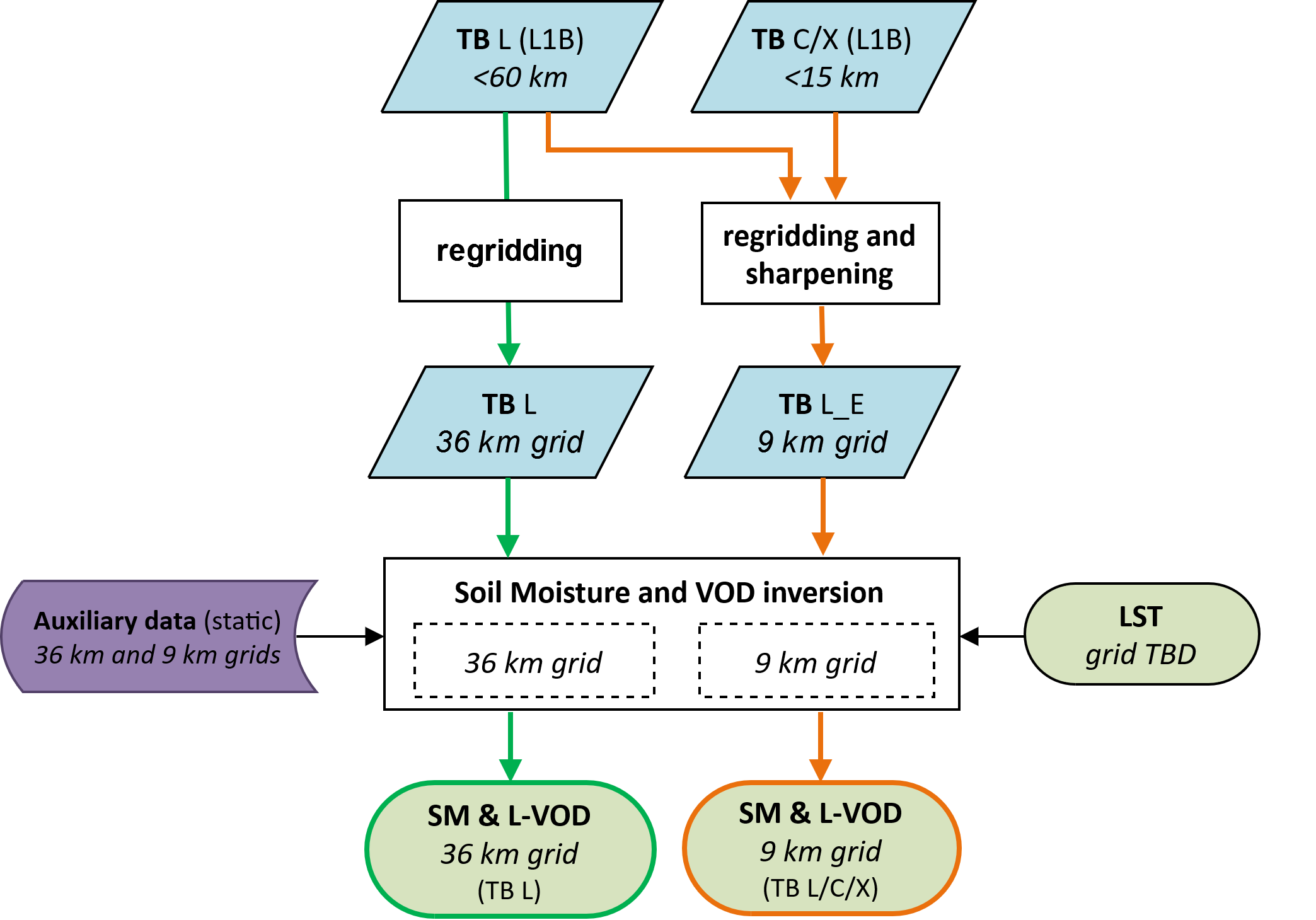
Fig. 4 Functional flow diagram of Level-2 Soil Moisture and VOD retrieval algorithm.

Functional description of each Algorithm step

Pre-processing of input TB

The processing algorithm primarily relies on the CIMR L1B TB product, which is calibrated, geolocated and undergoes several corrections, such as atmospheric effects, Faraday rotation and RFI effects. L, C, and X-bands are used as inputs to the Soil Moisture and VOD inversion. At each of these frequencies, fore- and aft-look TB data are merged and corrected for the presence of standing water. L-band undergoes an optimal interpolation or image reconstruction step (at the RGB toolbox). This product, TB_L, is directly used as input to the Level-2 retrieval algorithm to obtain the SM and L-VOD at coarse resolution (<60 km). TB_L is also combined with C-band or X-band TBs into an enhanced-resolution product TB_L_E, that is used as input to the Level-2 algorithm to obtain SM and L-VOD at an enhanced spatial resolution (~15 km).

Analyze surface quality and surface conditions

Ancillary data will be employed to help to determine whether masks are in effect for strong topography, urban, snow/ice, frozen soil.

Input data

The input data for the model consists of two primary parameters. The first is the Level 1b Brightness Temperature (L1B TB), which is observed by CIMR at L, C, and X-bands, covering both horizontal and vertical polarizations. This data represents a full swath or swath section with dimensions (Nscans, Npos) in a 2D array format. The second parameter, TB\(_{err}\), represents the error associated with the Brightness Temperature. This error information is also organized with the same dimensions, (Nscans, Npos).

More details can be found in the IODD.

Output data

The model outputs include key parameters such as soil moisture and vegetation optical depth at both the L-band (< 60km) and the L-band enhanced (~ 15km) resolution. The output data is produced in two nested EASE2 grids of 36 km and 9 km. Additional information like brightness temperatures and data flags supplement these outputs. Data flags enable users to examine the surface conditions of a grid cell and the quality of soil moisture estimate when retrieval is attempted.

More details can be found in the IODD.

Auxiliary data

Two sets of land surface temperature are planned to be included as auxiliary data for CIMR: the one estimated from CIMR Ku/Ka bands and the one from ECMWF. This will allow for some flexibility in the design and validation phase of the algorithm prototype. Until the CIMR land surface temperature retrievals are tested to serve as an input for soil moisture retrievals, the ECMWF dataset remains the first priority as an auxiliary dataset.

The static global maps for CIMR H and ω are computed through a weighted method. This approach takes into consideration the fraction of the MODIS IGBP land cover class that is contained within a given CIMR pixel. The data used for these computations are derived from the IGBP classification as identified in the study conducted by Fernandez-Moran [Fernandez-Moran et al., 2017]. In Table 3, different values of ω and \(H\) are listed according to land cover type. Based on these criteria, static global maps of ω and \(H\) have been produced as part of the ancillary dataset.

Table 3 Values of ω and \(H\)

ID	MODIS IGBP land classification	SMAP MTDCA ω	SMAP DCA ω	CIMR ω	SMOS-IC \(H\)	CIMR \(H\)
1	Evergreen Needleleaf Forests	0.07	0.07	0.06	0.30	0.40
2	Evergreen Broadleaf Forests	0.08	0.07	0.06	0.30	0.40
3	Deciduous Needleleaf Forests	0.06	0.07	0.06	0.30	0.40
4	Deciduous Broadleaf Forests	0.07	0.07	0.06	0.30	0.40
5	Mixed Forests	0.07	0.07	0.06	0.30	0.40
6	Closed Shrublands	0.08	0.08	0.10	0.27	0.27
7	Open Shrublands	0.06	0.07	0.08	0.17	0.10
8	Woody Savannas	0.08	0.08	0.06	0.30	0.40
9	Savannas	0.07	0.10	0.10	0.23	0.23
10	Grasslands	0.06	0.07	0.10	0.12	0.50
11	Permanent Wetlands	0.16	0.10	0.10	0.19	0.19
12	Croplands - Average	0.10	0.06	0.12	0.17	0.40
13	Urban and Built-up Lands	0.08	0.08	0.10	0.21	0.21
14	Crop-land/Natural Vegetation Mosaics	0.09	0.10	0.12	0.22	0.50
15	Snow and Ice	0.11	0.00	0.10	0.12	0.12
16	Barren	0.02	0.00	0.12	0.02	0.10

Furthermore, a CIMR Hydrology Target mask, applied in Level-2 data processing, provides a ≤1 km resolution and covers both permanent and transitory inland water surfaces. The mask incorporates data from the MERIT Hydro [Yamazaki et al., 2019] and the Global Lakes and Wetlands Database [Lehner and Döll, 2004], and it will be updated up to four times annually to account for potential seasonal changes.

The scene flag incorporates information about RFI, proximity to water body, urban, ice/snow, frozen soil, precipitation, dense vegetation, medium and strong topographic effects.

The rest of datasets that complement the ancillary information are the clay fraction (from FAO), a Land Cover Classification, and a Digital Elevation Model (e.g. from the Shuttle Radar Topography Mission (SRTM) [Jarvis et al., 2006, Mialon et al., 2008]).