Sea Ice Thickness Retrieval Algorithm

Introduction

The retrieval uses the fitted parameters from individual fits of ice thickness to brightness temperatures and a minimization scheme including uncertainties using the error covariance matrix of \(T_{b,h}\) and \(T_{b_v}\) at 1.4 GHz. In contrast to the original [Huntemann et al., 2014] retrieval, the upper limit is not capped but left open, but very loosely constrained by a background ice thickness. In the following the original fit parameters from [Huntemann et al., 2014] in the latest version are used for comparison and evaluation. However, the original parameters where obtained for an incidence angle range from 40° to 50° while the new fit parameters were obtained to match the CIMR incidence angle of 53°. The equations used for their fits are (3) and (4). Equation (3) is also used for fitting horizontal and vertical polarization directly to the ice thickness dependence. The inversion of this system in the \(H\) and \(V\) space is used to obtain the ice thickness. Both, \(T_{b,h}\) and \(T_{b_v}\) were fitted to the ice thickness dependence in the Forward model.

Retrieval definition

The retrieval is following a typical scheme with the objective to minimize

(9)\[ χ^2(\mathbf y,\mathbf x,\mathbf S_e,\mathbf S_a,\mathbf x_a)=\left(\mathbf y-F(\mathbf x)\right)^\mathbf{T}\mathbf S_e^{-1}(\mathbf y-F(\mathbf x))+(\mathbf x_a-\mathbf x)^{\mathbf T}\mathbf S_a^{-1}(\mathbf x_a - \mathbf x) \]

where \(\mathbf y= \begin{bmatrix}T_{b,h}\\T_{b,v}\end{bmatrix}\) is the vector of input (measured) brightness temperatures at L-band, \(\mathbf x\) is the result vector (in case of the retrieval of only one quantity, ice thickness, this is a scalar), \(\mathbf S_e\) is the error covariance matrix of the input brightness temperatures, \(\mathbf S_a\) is the covariance matrix of the background values (in this case a scalar), \(\textbf x_a\) is the background value (ice thickness) and \(F\) is the forward operator, in our caes the individual fit function for a given ice thickness, i.e., \(F(\mathbf x) = \begin{bmatrix}f_h(\mathbf x)\\ f_v(\mathbf x)\end{bmatrix}\), with \(f_p(x)\) from (3) and the corresponding parameters coming from Table Table 1.

The optimal solution \(\hat {\mathbf y}\) which minimizes equation (9) is found by iteration. The uncertainty of \(\mathbf y\) can then be obtained as

(10)\[ \mathbf {\hat S}_a= (\mathbf S_a^{-1}+\mathbf{ \hat M}^\mathbf T \mathbf S_e^{-1}\mathbf {\hat M})^{-1}, \]

with \(\mathbf {\hat M}\) is the Jacobian of the optimal solution of (9) which is in this case also a scalar.

Some variables are fixed in this scheme, this is the background ice thickness \(\mathbf x_a=x_a=100\) cm and its variance \(\mathbf S_a=S_a=20000\ cm^2\), which is used here as a practical way to very loosely constrain the upper ice thickness range. Other parameters are obtained from the CIMR satellite like \(\mathbf y= \begin{bmatrix}T_{b,h}\\T_{b,v}\end{bmatrix}\), the brightness temperatures at L-band, and the diagonal components of the error covariance matrix \(\mathbf S_a\), for the off-diagonal of \(\mathbf S_a\) there is no good estimate, but it is not expected that the uncertainties of \(T_{b,h}\) and \(T_{b,v}\) are uncorrelated. At least most physical effects which are not considered in this empirical forward model, would have to go into the uncertainty of \(T_{b,h}\) and \(T_{b,v}\) which introduce correlation. For the lack of a better estimate, we claim a correlation of 0.6 which results in off-diagonal elements of \(0.6*\sigma_{Tbh}\sigma_{TBv}\). For illustration of the algorithm we use

(11)\[\begin{split} \mathbf S_e = \begin{bmatrix}25 & 15\\ 15 & 25\end{bmatrix} \end{split}\]

For the minimization of (9) we use the Levenberg-Marquardt algorithm as described by [Rodgers, 2000] and [Marquardt, 1963]. An implementation in the Julia programming language [Bezanson et al., 2017] can be found below.

Show code cell source Hide code cell source

function lm_retrieval(Ta,Sₑ,Sₐ,xₐ,F)
    #Levenberg Marquardt method after Rodgers (2000)
    #target: find x so that F(x)=Ta, given
    #Ta: measurement vector
    #Sₑ: error covariance of measurement
    #Sₐ: error covariance of physical state 
    #xₐ: expected physical state (also used as start, i.e. first guess)
    #F: the forward model translating measument space into state space
    Sₐ⁻¹=inv(Sₐ)
    Sₑ⁻¹=inv(Sₑ)
    #function to minimize with changing input x
    J(y,x,Sₑ⁻¹,Sₐ⁻¹,xₐ,F)=(y.-F(x))'*(Sₑ⁻¹*(y.-F(x)))+(xₐ.-x)'*(Sₐ⁻¹*(xₐ.-x)) 
    xᵢ=copy(xₐ)
    Jᵢ=J(Ta,xᵢ,Sₑ⁻¹,Sₐ⁻¹,xₐ,F)
    γ=1e-5 #set to 0 for gauss newton
    for i=1:2000 
        Kᵢ=ForwardDiff.jacobian(F,xᵢ)
        Ŝ⁻¹=Sₐ⁻¹+Kᵢ'*Sₑ⁻¹*Kᵢ #eq 5.13
        xᵢ₊₁=xᵢ+((1+γ)*Sₐ⁻¹+Kᵢ'*Sₑ⁻¹*Kᵢ)\(Kᵢ'*Sₑ⁻¹*(Ta-F(xᵢ))-Sₐ⁻¹*(xᵢ-xₐ)) #eq 5.36
        Jᵢ₊₁=J(Ta,xᵢ₊₁,Sₑ⁻¹,Sₐ⁻¹,xₐ,F)
        d²=(xᵢ-xᵢ₊₁)'*Ŝ⁻¹*(xᵢ-xᵢ₊₁) #eq 5.29
        if Jᵢ₊₁<Jᵢ 
            γ/=2
        else
            γ*=10
            continue
        end
        xᵢ=xᵢ₊₁
        if d²<1e-10
            break
        end
        Jᵢ=Jᵢ₊₁
    end
    Kᵢ=ForwardDiff.jacobian(F,xᵢ)
    Ŝ=inv(Sₐ⁻¹+Kᵢ'*Sₑ⁻¹*Kᵢ) # eq 5.38
    
    return xᵢ,Ŝ
end


retrievallm(h,v)=first.(lm_retrieval(SA[h,v],SA[25 15;15 25.0],SMatrix{1,1,Float64,1}(20000.0),SA[100.],Fw_TB))

The comparison will be done with a least squares fit based \(I\)-\(Q\)-retrieval from Huntemann et al. 2014, i.e., the cost function is

(12)\[ c(x)=(I(x)-I_m)^2+(Q(x)-Q_m)^2 \]

which is minimized to obtain the best ice thickness \(x\) for a given measured \(I_m\) and \(Q_m\) and cap the result at 50 cm SIT as the stabilizing background term is missing.

Uncertainties

The uncertainty follows [Paţilea et al., 2019] using three terms:

• Uncertainty from the training data ice thickness increase within one day

• Native uncertainty from the of uncertainty of brightness temperatures

• Uncertainty from the ice concentration (not full ice coverage)

Technically, these uncertainties should be considered forward model errors and treated as such.

Daily ice thickness variation

Fig. 6 shows the SIT uncertainty from daily ice thickness variations from (1) for three different reference temperatures. For the following we use \(-25\ \text{°C}\) as uncertainty reference for contribution to the combined error calculation. Rearranging (1), for a fixed temperature, the cumulative freezing degree days to reach a certain ice thickness is

\[t_{\text{S}}(\text{d}_{\text{ice}},T)=-(\text{d}_{\text{ice}}/1.33)^{(1/0.58)}/(T+1.8) \]

(13)\[ \sigma_{\text{growth}} = 0.68\ (d_{\text{ice}}(t_\text{S}+1\ \text {day})-d_{\text{ice}}(t_\text{S})) \]

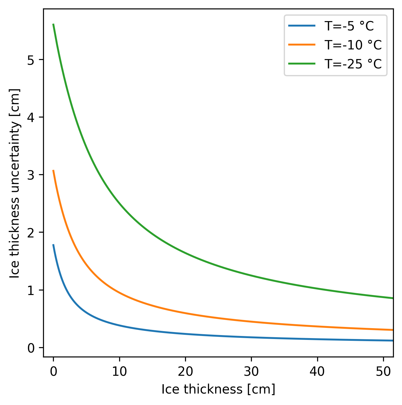
Fig. 6 Daily SIT increase at different temperatures and thicknesses

Propagation of brightness temperature uncertainty

The uncertainty of the CIMR brightness temperatures propagate into uncertainty in the retrieval natively. These are described by equation (10) and they are a direct result of the sensitivity of the forward modeled brightness temperatures to changes in physical parameters.

Uncertainty from full ice cover assumption

The assumption of full sea ice coverage within the CIMR L-band footprint originates from the unknown ice concentration. It can occur that a part of the footprint is open water, which lowers the brightness temperature and thus make the ice look thinner. This error is accounted for with a \(5\ \%\) error on ice concentration. The \(p_1\) for each parameter in Table 1 gives the open water tie point, i.e. at 0 cm ice thickness. For estimating the uncertainty, these values are mixed with the weight of the ice concentration as

\[ T_{b,h/v}(\text{SIC})=T_{b,h/v}\text{SIC} + p_{1,h/v}(1-\text{SIC})\]

so that

(14)\[ σ_\text{SIC} = \frac{F^{-1}\left(T_{b,h/v}(0.95)\right)+F^{-1}\left(T_{b,h/v}(1.05)\right)}{2} \]

Total uncertainty

The overall uncertainty is calculated as a composition of individual uncertainties in the parameter space, i.e. on ice thickness directly as

(15)\[ σ_\text{tot}=\sqrt{\left(σ_{\text{SIC}}^2+σ_\text{growth}^2 + \sigma_\text{retr}^2\right)}, \]

assuming they are uncorrelated. The indiviual terms as well as the total uncertainty are shown in Fig. 7 on the left. At small ice thicknesses, the largest contribution is from the ice growth error up to about \(15\ \text{cm}\). From there, the sensitivity to changes in ice thickness gets smaller and the uncertainty from the SIC takes over the higher contribution. The retrieval error as the propagated brightness temperature uncertainty, shows the highest values only at higher ice thicknesses. On the right of Fig. 7 the relative error is shown. The best accuracy is reached at ice thicknesses between \(10\ \text{cm}\) and \(60\) cm with the relative error below \(40\ \%\).

Note

The ice concentration error is not a fixed function of the ice thickness as it is evaluated in the brightness temperature space and thus depends on the input brightness temperatures.

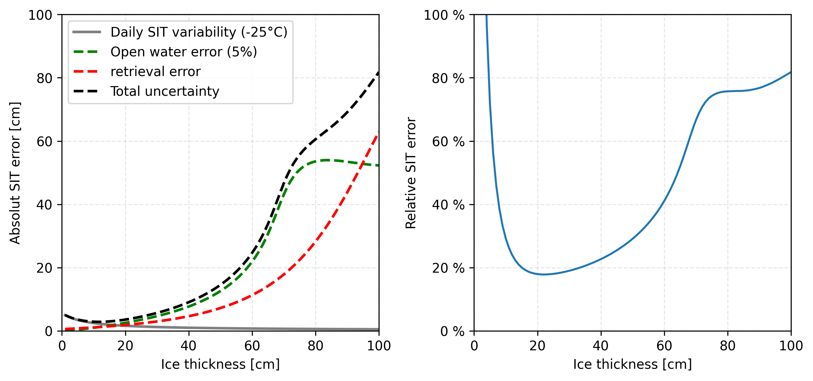
Fig. 7 Influence of different error terms on SIT error caculation. Left: absolute error, in dashed is the new implementation described here. Right: relative error for given ice thickness.

The overall retrieval SIT for a given combination of \(T_{b,h}\) and \(T_{b,v}\) is shown in a contour plot in Fig. 8. The dots represent the forward model evaluation for a given ice thickness in \(10\ \text{cm}\) steps, converted to \(I-Q\)-space. The orange dots are the CIMR algorithm described in this ATBD, the red dots correspond to the \(I-Q\) space fit variant from [Huntemann et al., 2014] and [Paţilea et al., 2019]. The bottom right dots show \(0\ \text{cm}\) ice thickness, where both function essentially give the same point. At the \(10\ \text{cm}\) up to \(40\ \text{cm}\) there is a slight discrepancy in the direction of polarization difference. Also, at higher SIT values the red points do not reach as high intensities and polarization difference as the orange points of the new retrieval.

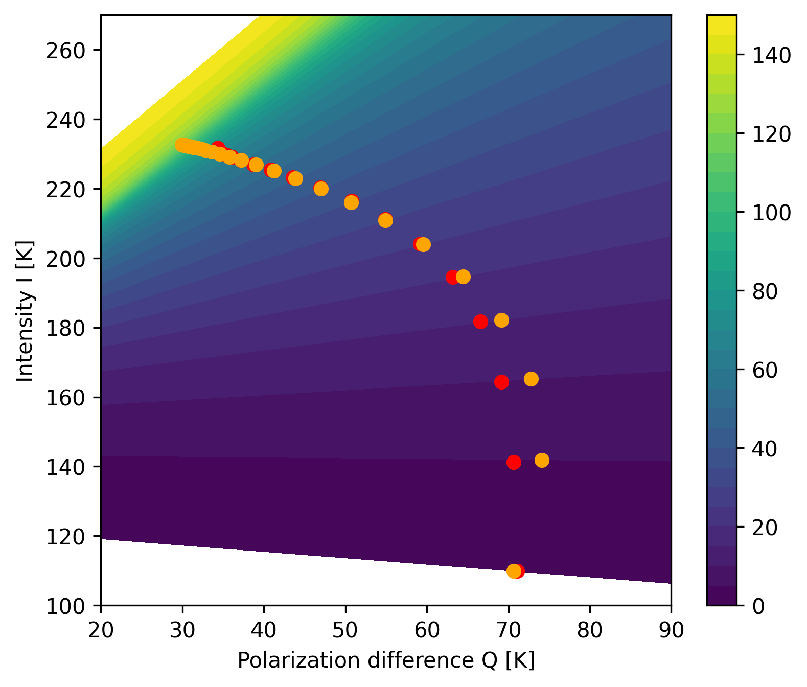
Fig. 8 r”Display of retrieval function in \(I\)-\(Q\)-space. Orange dots show the forward function \(I\) and \(Q\) for a given ice thickness in 10cm steps, blue dots are from an actual \(I\)-\(Q\) fit.”