Forward model

Introduction

The training data was generated in [Huntemann et al., 2014]. It consists of modeled ice thickness increase from a cumulative freezing degree day model for the freeze-up in 2010 in the Kara and Barents Seas. In this document we are using the data from SMOS which, like CIMR observes brightness temperatures at L-band and the cumulative freezing degree day model to fit an analytic equation to the dependency of brightness temperature and ice thickness. In contrast to [Huntemann et al., 2014], here instead of the Intensity and Polarization difference, the horizontal and vertical polarized brightness temperatures are used directly.

Fit from a sea ice thickness dataset

An empirical model of the ice thickness increase was proposed with the so-called cumulative freezing degree days [Bilello, 1961]. The idea is that the integration of negative air temperatures over time is a proxy for the physical ice thickness increase. The original formulation is

(1)\[ d_{\text{ice}}(\Theta) = 1.33{\Theta}^{-0.58} \]

(2)\[\Theta = \sum_{\text{days}} T_{\text {air}}+1.8\ {}^\circ \text C \text , \]

with \(T_{air}\) being the daily average air temperature. The exponent of \(\Theta\) in equation (1) was found to vary depending on the location, snow accumulation and wind and cloud conditions [Bilello, 1961]. The air temperature used to calculate for \(\Theta\) here originate from NCEP/NCAR reanalysis [Kalnay et al., 1996]. The 1.8° C offset is here to compensate for the freezing temperature of sea water at typical salinities.

The dataset was acquired in 2010 in the Kara and Barents Seas. The dataset here is treated differently compared to [Huntemann et al., 2014] in two points

• From the initial 10 small subregions only regions 3, 6, and 7 were used to obtain the original fit parameters, here all regions are used.

• The original retrieval removed the 0 cm ice thickness, i.e., open water cases in the fit, due to instability in fitting procedure for the polarization difference \(Q\), these open water points are now included here.

The extraction of brightness temperature for the fit procedure and algorithm development had to be re-evaluated at an incidence angle of 53° for this document since the incidence angle for previous fit attempts where different with [Huntemann et al., 2014] being 40°-50° average, and [Paţilea et al., 2019] using 40°.

Note

The actual incidence angle of CIMR at L-band is closer to 52° than to 53°. The fit here in this ATBD is still optimized for 53° which is partly compensated by the Correction for variation in incidence angle.

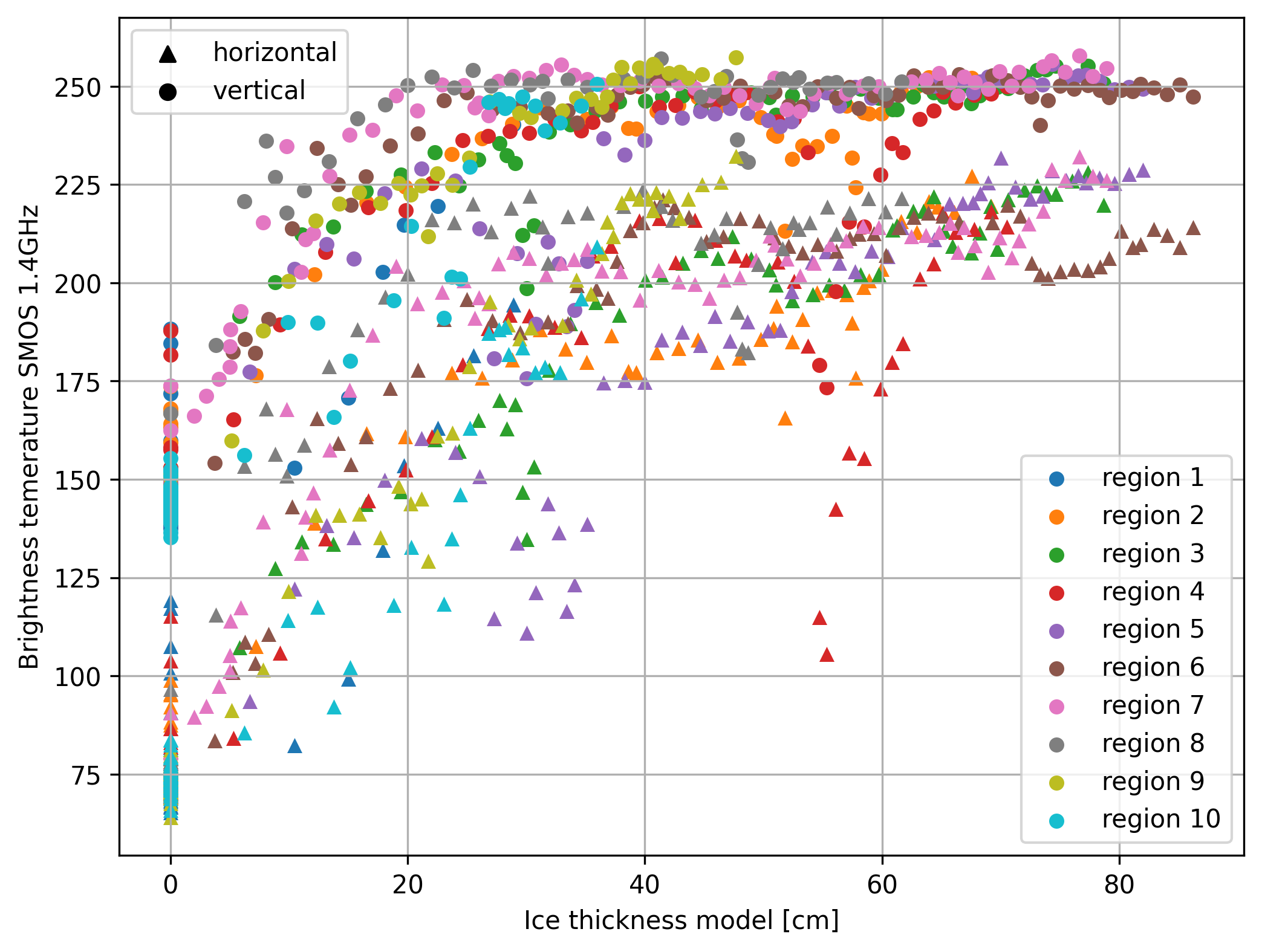
Fig. 1 Ice thickness to brightness temperature relation showing the original SMOS data for the three resions from [Huntemann et al., 2014] extracted at 53° incidence angle.

Fig. 1 gives a nice relation between ice thickness and the brightness temperatures in horizontal and vertical polarization. Horizontal shows a slower increase and later saturation but is subject to more noise in general. For the fitting procedure 0 cm ice thickness, i.e. open water, is included. The individual regions are shown in Fig. 2. The regions in Fig. 1 and Fig. 2 are corresponding according to their color. Most regions are located East to North-East of Novaya Zemlya in the Kara Sea but some regions are also located North-West of Novaya Zemlya in the Barents Sea.

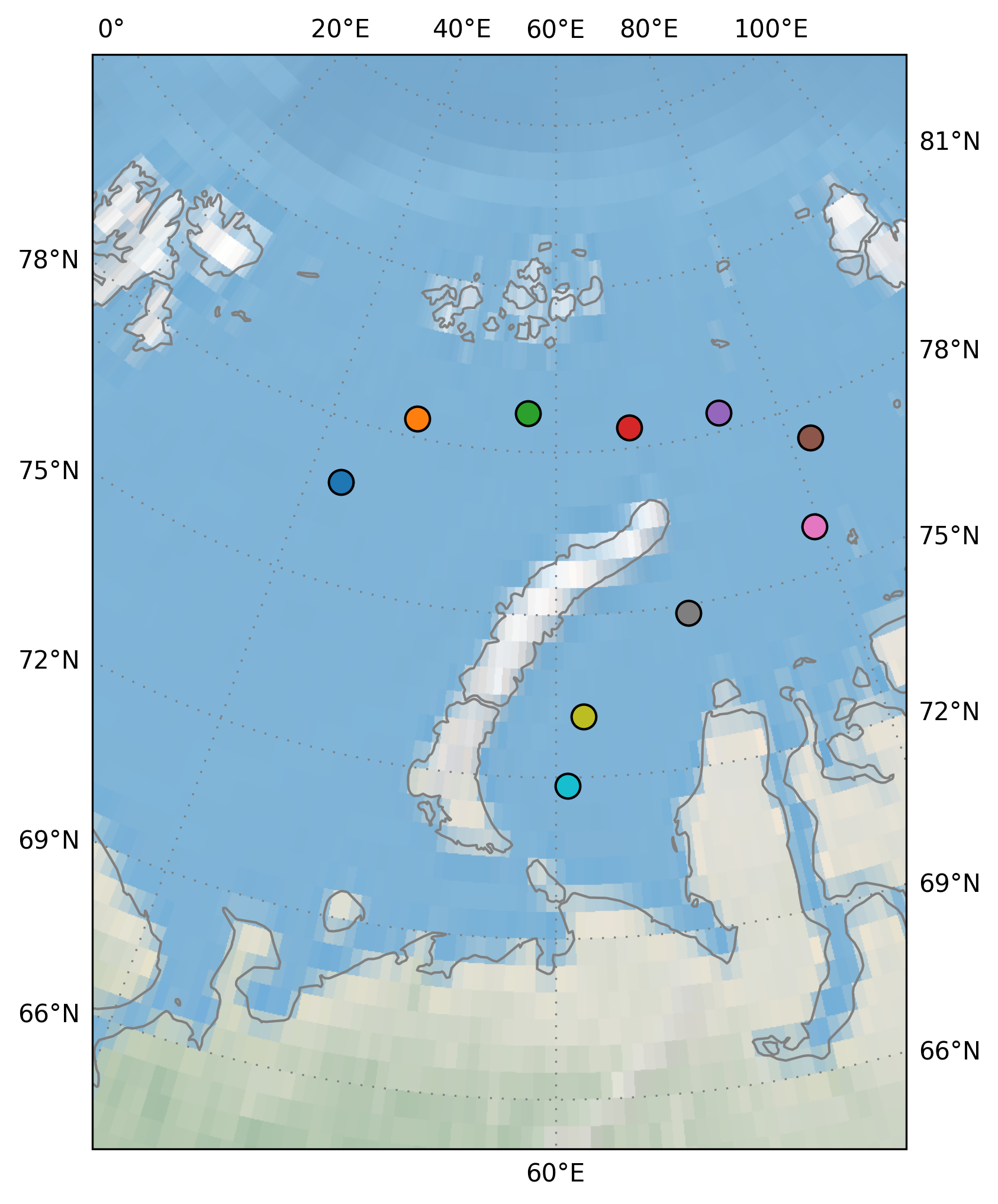
Fig. 2 Regions in the Kara and Barents Seas from the 2010 training data.

Parameter estimation

As a fit function a simple exponential is used with

(3)\[ f_p(x)= p_2 - (p_2 - p_1)\exp(-x/p_3) \]

where \(p_1\) is effectively the brightness temperature of open water close to sea ice under freezing conditions, \(p_2\) is the brightness temerature of thick sea ice, and \(p_3\) is a curvature parameter connecting the two TBs. The index \(p\) of \(f_p\) indicates the polarization, either \(h\) or \(v\).

The parameters \(p_i\) are optained in a fit to the data from the ten regions mentioned. A least square fit of equation (3) for \(T_{b,h}\) and \(T_{b,v}\) individually gives 6 parameters in total. The same can be done in intensity and polarization difference space while for polarization difference another fit formula is used

(4)\[ f_Q(x)= p_2 - (p_2 -p_1)\exp(-(x/p_3)^{p_4}) \]

To compare the ice thickness to brightness temperature relation based on the new fit parameters, the original fit parameters have to be recalculated for the 53° incidence angle of CIMR. This gives 7 parameters for the recalculation of the original fit, with an additional parameter \(p_4\) for the polarization difference fit. The fit parameters are given in Table 1.

Table 1 Fit parameters for intensity and polarization difference

parameter	\(p_1\)	\(p_2\)	\(p_3\)	\(p_4\)
horizontal \(T_{b,h}\)	74.527	217.795	21.021
vertical \(T_{b,v}\)	145.170	247.636	12.509
intensity \(I=(T_{b,v}+T_{b,h})/2\)	109.891	231.596	16.829
polarization difference \(Q=(T_{b,v}-T_{b,h})\)	71.086	34.322	38.731	2.142

Comparison between \(I-Q\) and \(h-v\) fit

A resulting fit through all data points show that also the direct horizontal and vertical fits are suitable for representation of ice thickness to brightness temperature relation, similar to the originally \(I-Q\) fit from [Huntemann et al., 2014]. The fit parameters are given in Table 1. The comparison of a \(I-Q\) fit and a \(T_{b,v} - T_{b,h}\) fit is shown in Fig. 3. Only a slight difference is seen in \(T_{b,h}\) at higher ice thickness.

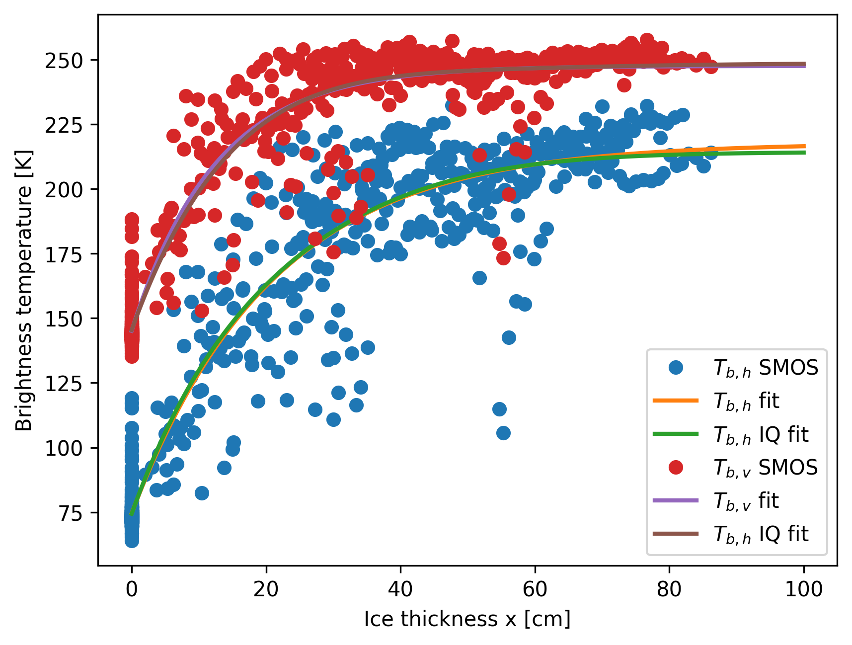
Fig. 3 Comparison of brightness temperature fits for horizontal and vertical polarizations against ice thickness.

The relation for polarization difference, i.e. \(T_{b,v} - T_{b,h}\) to ice thickness, shows also good agreement with the data in both fit variants in Fig. 4. However, some differences are visible for thin ice and in the extrapolation to higher thicknesses. The increase of polarization difference after the initial freeze-up, between 5 cm and 10 cm ice thickness, seems physically plausible as calming of seawater results in smaller sea surface roughness and thus increased polarization difference. This is not captured by the \(I-Q\) fit functions as the (4) is constrained in this regard.

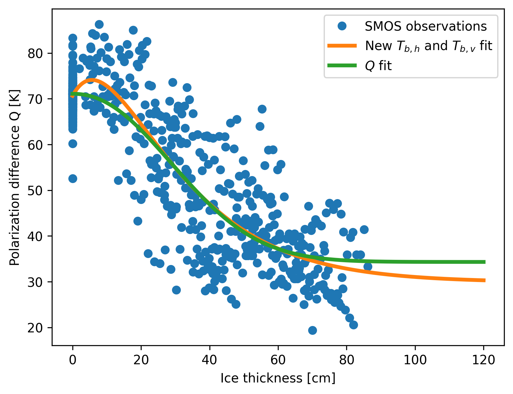
Fig. 4 Comparison of polarization difference fits against ice thickness.

The polarization difference plotted versus intensity, which is the original representation used by [Huntemann et al., 2014] and [Paţilea et al., 2019] also shows that the fit is appropriate in the \(I-Q\)-space in Fig. 5. The most notable difference is the same as in the Fig. 4 figure, i.e. the increase of polarization difference after the initial freeze-up, in the 5-10 cm regime. The highest ice thickness displayed here is 120 cm, which is a extrapolation for the current fit and comes with an extra uncertainty.

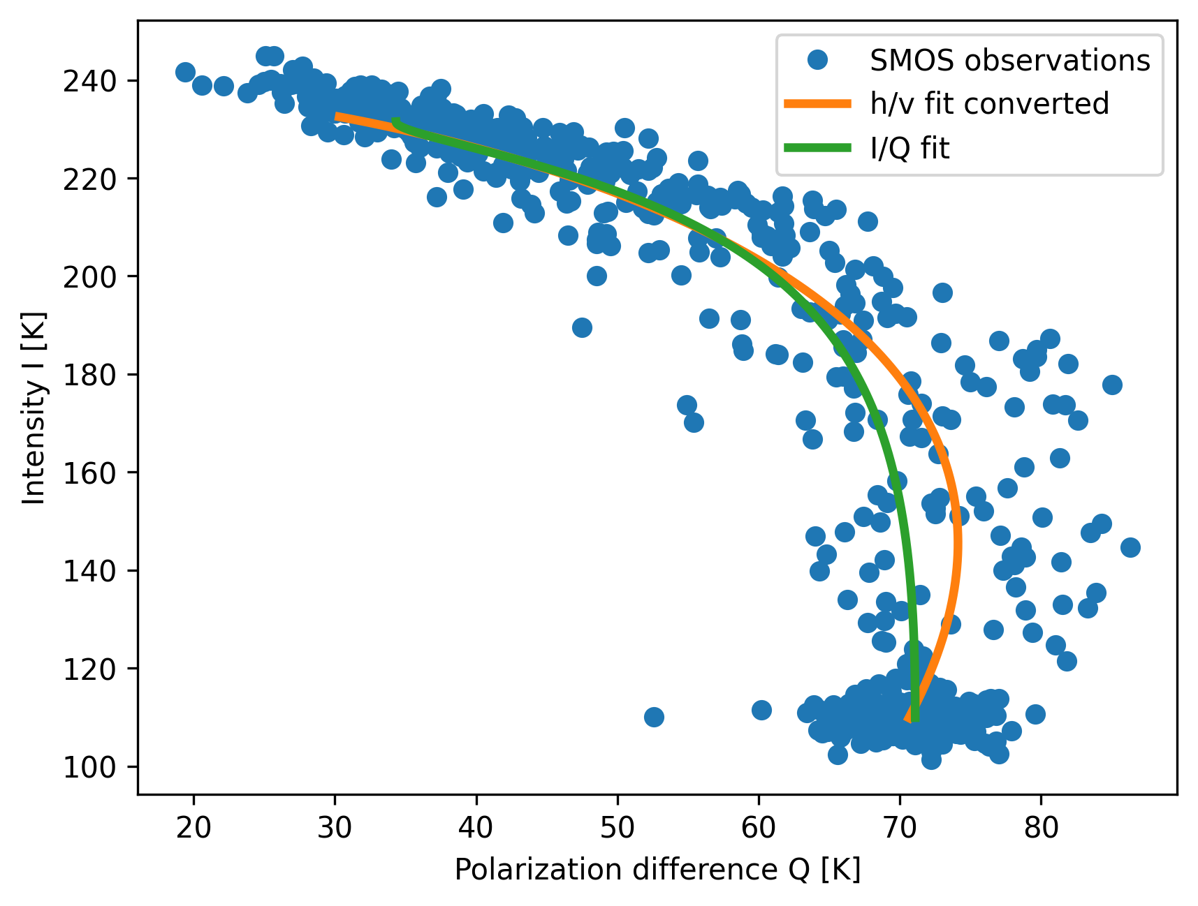
Fig. 5 Comparison of fits in intensity vs. polarization difference space.

Correction for variation in incidence angle

While the algorithm is designed for a fixed incidence angle, the incidence angle is varying slightly depending on the feed horn which is used for the observation which, in turn, changes the brightness temperatures. We attempt a straightforward correction for the incidence angle dependence of the brightness temperatures by estimating the surface reflectivity using the polarization information for a given observation. The assumption here is a simple Fresnel reflection model without an atmospheric contribution. First, we define the Fresnel reflection coefficient of the surface with given effective permittivity \(\varepsilon\) and incidence angle \(\theta_i\) as

(5)\[\begin{split}E_{0p} &= 1-|r_p|^2\\ r_v &= \frac{ε\cos(θ_i)-\sqrt{ε-\sin^2(θ_i)}}{ε\cos(θ_i)+\sqrt{ε-\sin^2(θ_i)}}\\ r_h &= \frac{\cos(θ_i)-\sqrt{ε-\sin^2(θ_i)}}{\cos(θ_i)+\sqrt{ε-\sin^2(θ_i)}}\end{split}\]

The effective permittivity is used here which is a simplification calculated with the assumption that the atmosphere is transparent. We use an effective surface temperature \(T_{\text{eff}}\) which we set to \(T_{\text{eff}}=240\) if \(T_{b,v}<220\) K otherwise it is set to \(T_{\text{eff}}=T_{b,v}+20\) K as an approximation. Then we have

(6)\[T_{\text{eff}} = \frac{T_{b,h}(θ_i) \cdot (1-r_h(ε,θ_i)) + T_{b,v}(θ_i)\cdot(1-r_v(ε,θ_i))}{2}\]

which we can solve for a given \(θ_i\) to get the effective permittivity as

(7)\[ε_{\text{eff}} = \operatorname{arg\,min}_{ε \in \mathbb{R}} \left| \left( \frac{T_{b,h}(θ_i)}{T_{\text{eff}}} - (1-r_h(ε,θ_i))\right)^2 + \left( \frac{T_{b,v}(θ_i)}{T_{\text{eff}}} - (1-r_v(ε,θ_i))\right)^2 \right|\]

The corrected brightness temperature for the incidence angle \(θ_{\text{ref}}\) at vertical polarization is then given by

(8)\[T_{b,p}(θ_{\text{ref}}) = T_{b,p}(\theta) + \left(r_p(ε_{\text{eff}},θ_{\text{ref}}) - r_p(ε_{\text{eff}},θ)\right) \cdot ζ\]

with \(θ\) being the incidence angle of the observation. In theory, we expect the correction factor \(ζ\) to be equal to the effective temperature \(T_{\text{eff}}\) which approximately fits for L-band at both polarizations. This allows us to compensate the brightness temperatures for small variation in incidence angle, improving the accuracy of our ice thickness estimations.

CIMR Level-1b re-sampling approach

The CIMR Level-1b data is resampled using a nearest neighbor interpolation onto the output grid. Since the SIT retrieval only uses one single channel (L-band) there is no interpolation needed for bringing different frequencies together as input for the algorithm.

Algorithm Assumptions and Simplifications

The CIMR SIT algorithm described here is designed to be used in high sea ice concentration areas, with little to no open water contamination within the L-band footprint. This is not always the case, in particular at the ice edges. The impact of the sea ice concentration on the SIT retrieval is discussed in Influence of ice concentration against ice thickness underestimation. Similarly costal contamination is not considered in the algorithm and any form of costal influence within the footprint would show as higher sea ice thickness, as the brightness temperatures of land surfaces are closer to that of thick sea ice than to open water. As a consequence, the retrieval may show coastal contamination in the area around land surfaces which show up as increased ice thickness, creating the impression that all land surfaces are surrounded by thin sea ice. There are several way to deal with this effect in the final product

• External information about costal contamination of the L-band footprint which is currently not provided in the L1b data (depends on location and azimuth angle)

• Masking a region around land surface where the retrieval is not applied and the product yield NaN values (most conservative)

• Propagating closest valid values into regions close to coast, while the exact distance need to be determined from real CIMR data.

Level-2 end to end algorithm functional flow diagram

graph TD B[Input CIMR Level-1b data] --> C[Preprocess data] C --> D[Apply incidence angle homogenization] D --> E[Apply SIT retrieval] D --> F[Apply SIT uncertainty calculation] F --> H F --> G E --> G[Calculate flags] G --> H[Resampling to output L2 file] E --> H

Functional description of each Algorithm step

The processing chain works as follows:

1. Input CIMR Level-1b data: The algorithm begins by ingesting the raw Level-1b data from the CIMR satellite, which includes brightness temperature measurements at L-band frequencies.

2. Preprocess data: The data is preprocessed to remove any noise and correct for any known biases or errors in the measurements. This step may include filtering and calibration to ensure the data quality is suitable for further analysis.

3. Apply incidence angle homogenization: A correction is applied to account for variations in the incidence angle of the observations. This involves estimating the effective permittivity and adjusting the brightness temperatures based on the Fresnel reflection model (see Correction for variation in incidence angle)

4. Apply SIT retrieval: The SIT retrieval algorithm is executed, utilizing the corrected brightness temperatures to estimate the thickness of the sea ice. This step involves fitting the brightness temperature data to the established models for both horizontal and vertical polarizations (see Retrieval definition)

5. Apply SIT uncertainty calculation: Uncertainty estimates are calculated for the SIT retrievals, taking into account the variability in the input data and the assumptions made during the retrieval process (see Uncertainties).

6. Calculate flags: Flags are generated to indicate the quality of the retrievals, including any potential issues such as coastal contamination or low confidence in the SIT estimates.

7. Resampling to output L2 file: Finally, the processed data, including the SIT estimates, uncertainty values, and quality flags, are compiled into a Level-2 output file for further analysis and dissemination.