Evaluation on Simulated test scenes

In the CIMR DEVALGO project, we have developed a set of test scenes to evaluate the performance of the algorithms. The test scenes evaluated here in the SIT ATBD, are the Test scene 1 (radiometric scene), Test scene 2 (geometric scene) and the polar scene from the SCEPS project. The test scenes are simulated scenes with known ground truth, and are used to evaluate the performance of the algorithm. The test scenes are described in the following sections.

Test scene 1 (Radiometric scene)

The test scene 1 contains nine different surface classes, each with its own set of brightness temperatures. For the generation of these brightness temperatures a simple forward model was used, dependent on the surface type. Technically, the scene can be evaluated with unknown surface properties ignoring the surface classes. However, for an overview, these classes are shown in figure Fig. 15.

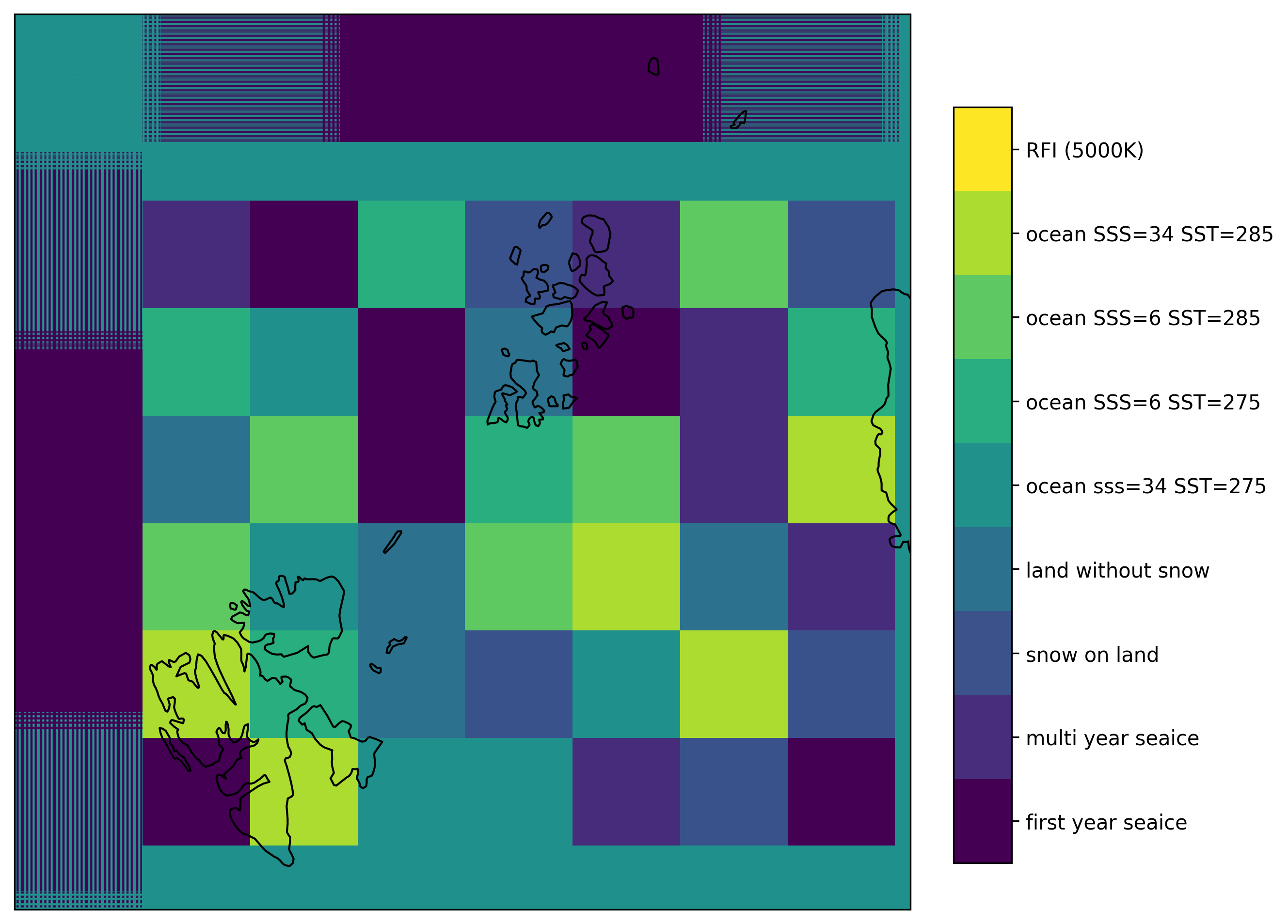
Fig. 15 Overview of surface types on Test Scene 1.

Fig. 16 shows the comparison between the retrieval applied to the brightness temperatures which where input to the satellite simulator on the left. This serves as ground truth for the scene 1 comparison. Here, no footprint or antenna pattern is taken into account and the resulting retrieval looks crisp and sharp. In the center, the retrieval on the output of the CIMR satellite simulator is shown. The pattern is smoothed out due to the footprint and antenna pattern. The retrieval is still able to retrieve the main features of the scene. The major difference is seen in the intermediate sea ice concentrations of about 50 % which are present in the stripes on the top and left border of the scene. These are retrieved as very thin ice (barely distinguishable from open water) due to the non-linearity of the retrieval. On the right, the difference between the two retrievals is shown. The difference is mainly due to the smoothing of the scene and the non-linearity of the retrieval. While mostly blue (underestimation of ice thickness), there is a slight hint of red (overestimation) at each edge. This is over open water where the footprint still sees some ice which then barely has any influence on the retrieval but only shifts it slightly above the 0 cm ice thickness which is retrieved for open water.

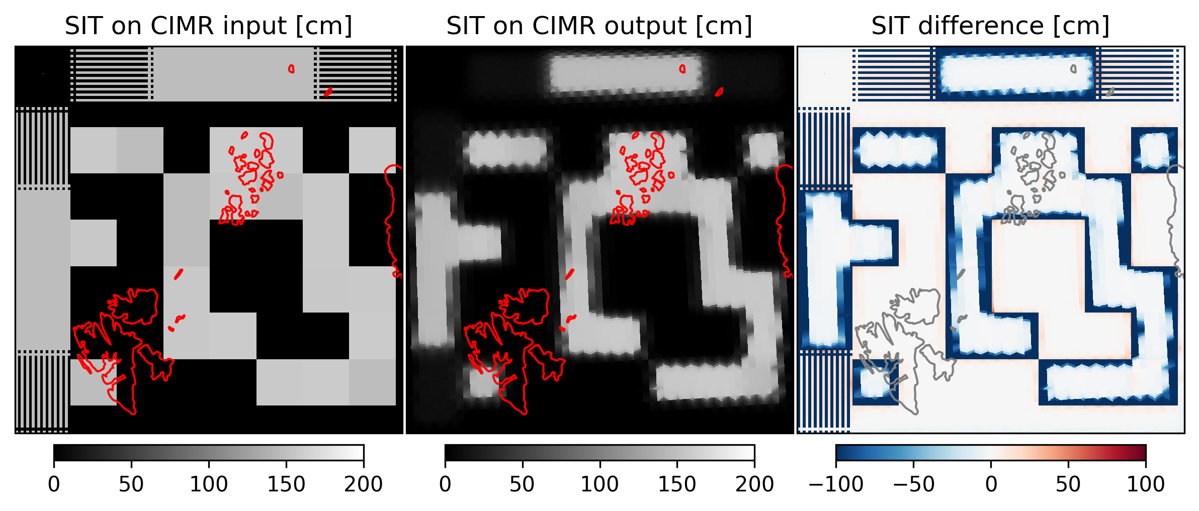
Fig. 16 Comparison of SIT retrieval on input to the CIMR satellite simulator (left) and on it’s output (center) together with their differences (right).

Since the CIMR satellite simulator distinguishes between the forward and backward scan, we can seperrate the retrieval into the two directions in Fig. 17. While in the original SIT retrieval (and brightness temperatures) the structures in scene 1 were strait, when selecting only forward or backward scan directions, the structures become curved depending on the the scan direction. This was not so much visible in Fig. 16 when both directions were combined, even though using only nearest neighbor resampling. This might also be due to the fact that in the L1b data which was taken as input, every sample along the scan line was available individually while having a physical overlap. In the planned L1b data format, five samples are combined to one, which might affect the impression of the scan line appearance. On the right side of Fig. 17 the retrieval uncertainty is shown. As can be seen, high ice thicknesses also yield high uncertainties, even larger than the ice thickness itself. This is due to the extension of the retrieval to the full range of possible ice thicknesses.

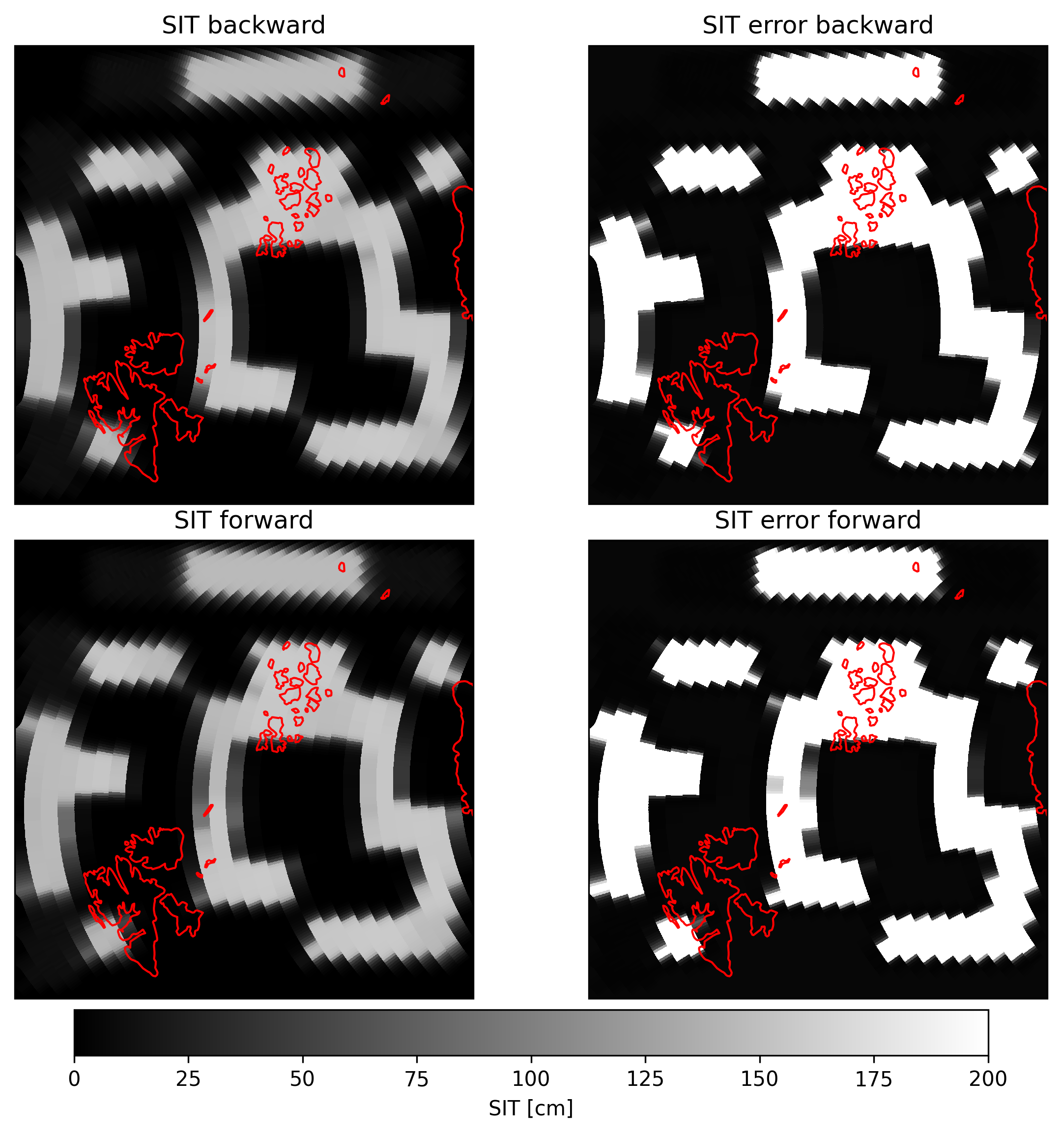
Fig. 17 SIT retrieval on the CIMR satellite simulator output for test scene 1 (radiometric scene).

Scene 2 (Geometric scene)

The scene 2 involves some star-like structures and circles which are seen nicely on the left side of Fig. 18. Only one ice type and ocean type is present in this scene, so the retrieval shows only two different values for the ice thickness with all details and sharp edges. In the center of Fig. 18 the retrieval on the CIMR satellite simulator output is shown. Here the influence of the footprint size of L-band is strongly influencing the result. The thin star-like structures on the bottom (ice on water background) are barely visible as their area fraction on an L-band footprint is very small. Also the non-linearity of the retrieval causes the strong underestimation of the ice thickness for the lower part of the scene. Likewise, in the upper part of the screen, the star-like structures (water on ice background) are expanding due to the non-linearity of the retrieval. The difference map on the right of Fig. 18 reflects this underestimation of ice thickness across the scene, again with a slight overestimation at the edges.

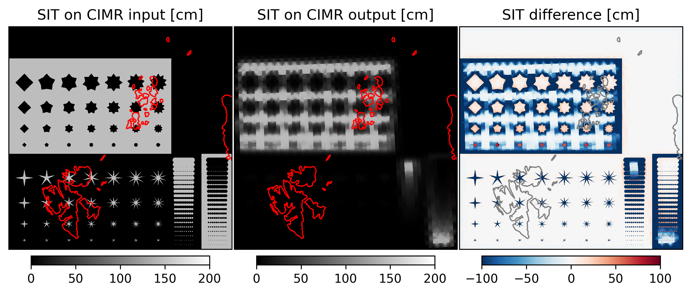
Fig. 18 Comparison of SIT retrieval on input to the CIMR satellite simulator (left) and on it’s output (center) together with their differences (right).

Comparing forward and backward scan for scene 2 in Fig. 19, the star-like structures are are not recognizable in their shape and take a curvy structure in each forward and backward scan. The retrieval uncertainty on the right side of Fig. 19 shows the same behavior as in scene 1, with high ice thicknesses yielding high uncertainties.

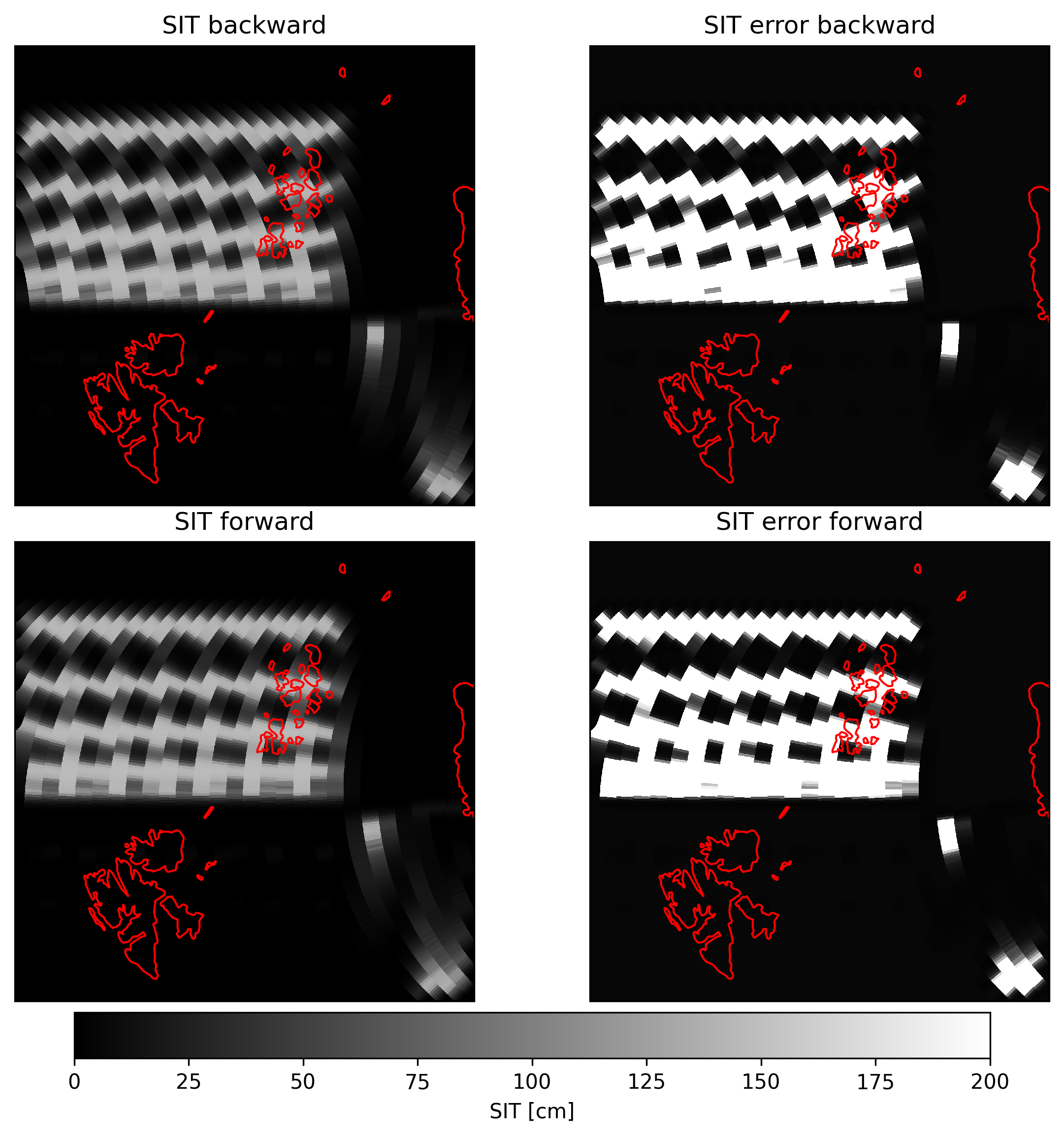
Fig. 19 SIT retrieval on the CIMR satellite simulator output for test scene 2 (geometric scene).

SCEPS polar scene

The SCEPS polar scene is located in the same region as the DEVALGO test scenes 1 and 2 but is based on model data and corresponding simulated brightness temperatures. The retrieval on the input brightness temperatures to the SCEPS CIMR satellite simulator is shown on the left side of Fig. 20. The structure contains unnatural curves but also resonable ice structures in particular around Franz Josef Land. The retrieval on the output of the CIMR satellite simulator is shown in the center of Fig. 20. The retrieval is able to retrieve the main features of the scene and in this scene the non-linearity of the retrieval is not that influential as on the other scenes as here, open water borderes thin ice areas, so that the effect of smoothing is reduced. The difference map on the right side of Fig. 20 shows the underestimation of ice thickness in the center of the scene and the overestimation at the edges and regime changes in ice thickness. A slight overestimation is visible in the thicker ice area, which could be due to a slight warm bias in the simulated brightness temperatures output of the CIMR satellite simulator.

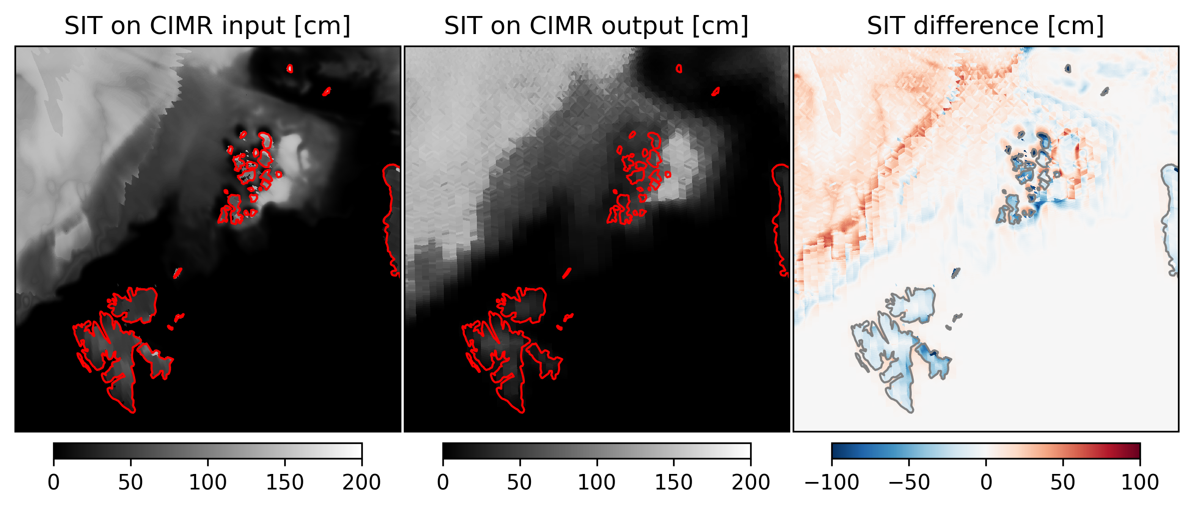
Fig. 20 Comparison of SIT retrieval on input to the CIMR satellite simulator (left) and on it’s output (center) together with their differences (right).

For completeness, we also compare the retrieval on the forward and backward scans of the the SCEPS polar scene in Fig. 21. In the forward scan, the scanline is alligned with the ice edge which gives an unnatural appearance to the ice edge. This is not that pronounced in the backward scan as the scannline is perpendicular to the ice edge. The retrieval uncertainty on the right side of Fig. 21 shows the same behavior as in the other scenes, with high ice thicknesses yielding high uncertainties. In general, also in the SCEPS polar scene, the combined forward and backward scan retrieval (Fig. 20 center) gives a more realistic appearance of the ice edge and more fine grained features than the individual forward or backward scan retrieval.

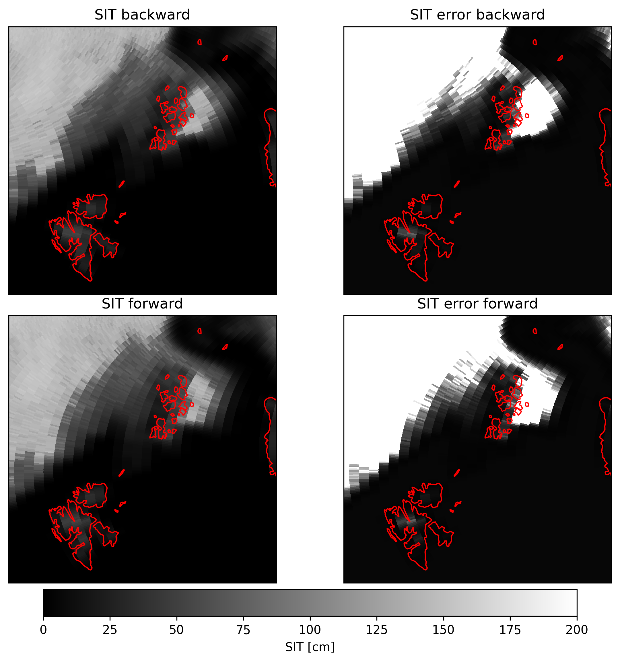
Fig. 21 SIT retrieval on the CIMR satellite simulator output for the SCEPS polar scene.

Comparison to reference data on SCEPS polar scene

The reference data for the polar scene is also provided from SCEPS and was used to simulate corresponding brightness temperatures which are input to the retrieval and to the satellite simulator. The reference SIT data is shown in Fig. 22 on the left side. The reference ice thickness seem reasonable with thin ice around Franz Josef Land and thicker sea ice towards the North pole. The retrieval output (same as in Fig. 20) is shown in the center of Fig. 22 together with the difference on the right. The major difference is seen in the underestimation of ice thickness in the center of the scene at the ice edge, but also the ice at Franz Josef Land is highly overestimated by the retrieval.

Note

Here the reference data set is not an absolute truth. We can only compare the retrieval to the reference data, but we cannot say which one is more accurate or closer to the truth.

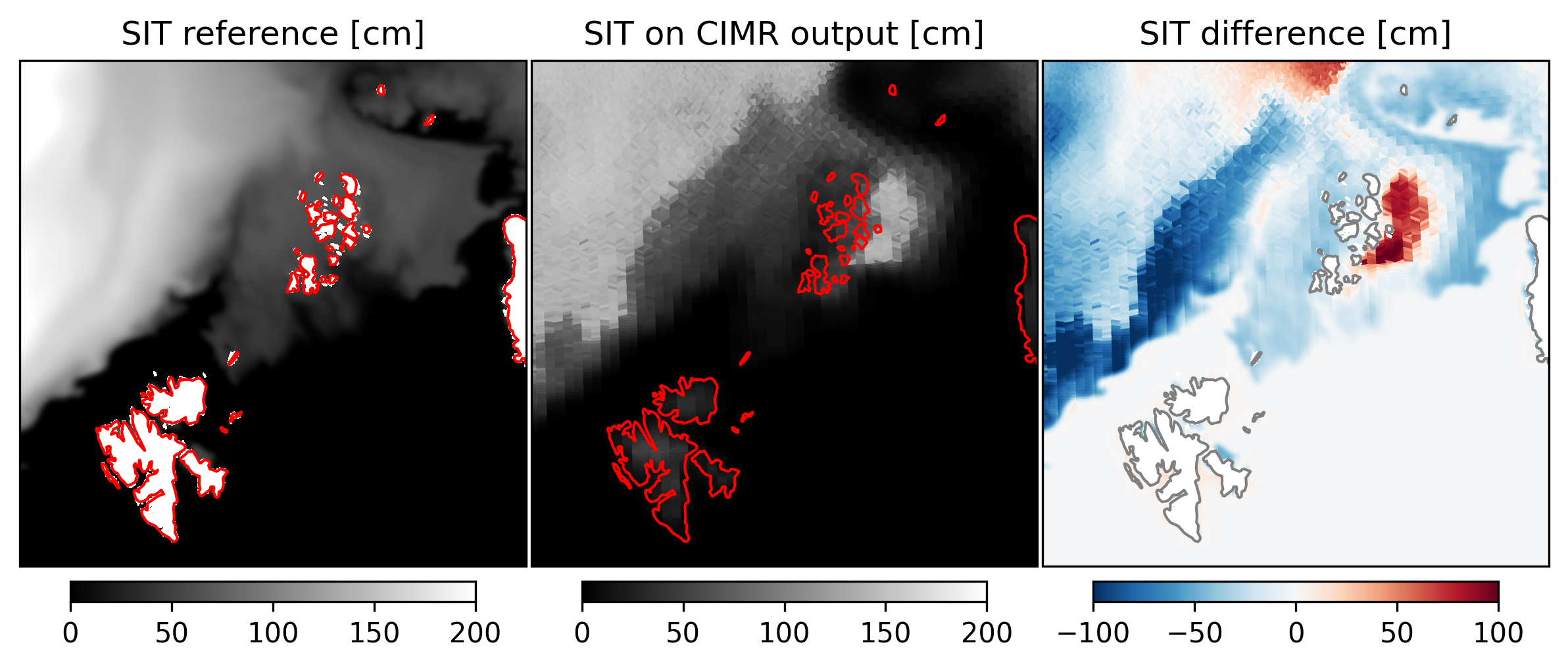
Fig. 22 Comparison of reference SIT on the SCEPS polar scene (left) and the retrieval applied to the SCEPS CIMR simulator (center) together with their differences (right).

Summary

In Table 2, the algorithm performance on input and output is compared by applying the algorithm to both, input and output TBs of the CIMR satellite simulator. Their difference is calculated and the mean and standard deviation of the difference is shown in the table together with the mean SIT of the scene. In addition, for the SCEPS polar scene, the reference SIT is used for the comparison in the last row of the table. In scene 1 and scene 2, the difference is negative on average, This is because there is mainly an underestimation of the SIT, as the satellite simulator smoothens the TBs and can create intermediate brightness temperatures. Over open water close to the ice edge, the SIT is overestimated, while over thick ice, close to open water the underestimation of the ice thickness is not tha pronounced.

Table 2 Performance comparison on the different scenes for the forward and backward comibined retrieval. The mean and standard deviation of the difference between the retrieved and the true SIT (retrieval on simulator input TBs or reference data set) is given.

Scene	mean true SIT [cm]	mean difference [cm]	std difference [cm]
Scene 1	75.05	-24.98	49.63
Scene 2	49.20	-25.91	48.58
Scene P	36.19	1.57	13.28
Scene P (reference)	54.46	-15.97	27.57

Special metrics

We have two special metrics, one is the evaluation of ice thickness underestimation against the distance to the closest water pixel and the other is the ice concentration within a certain radius against the ice thickness underestimation.

Ice thickness underestimation against distance to closest water pixel

As a special metric we compute the ice the ice thickness underestimation as a function of distance to closest water for the DEVALGO test scene 2 (the geometric scene). The distance to the closest water is calculated for each pixel together with the retrieved ice thickness. For each distance bin, the mean and the 10 and 90 percentile of the ice thickness is calculated and subtracted from the true ice thickness which is the fixed value of 148 cm of for the ice used in the scene. The result is shown in Fig. 23 (left). The underestimation of the ice thickness is decreasing with increasing distance to the closest water pixel. A strong drop of the underestimation is visible at a distance above 40 km which is likely related to the CIMR footprint size at L-band. At 60 km distance there is barely an underestimation of ice thickness even for the 90 percentile. The right side of Fig. 23 shows the used scene including all used pixels. The borders of 100 km width are removed because of the 0 K brightness temperatures which were used as input outside of the simulated scene, spreading into it due to the footprint size of the simulation.

Fig. 23 Left: SIT underestimation for thick ice as a function of distance to the ice edge for scene 2. Right: retrieved SIT on scene2, 100 pixel at the edges are removed.

Influence of ice concentration against ice thickness underestimation

He we compute the ice thickness underestimation as a function of ice concentration within a radius of 15 km and 50 km. To illustrate the ice concentration within a certain radius, we show the ice concentration within a radius of 15 km on the map in Fig. 24. The shape of the features is a bit blurry due to the 15 km radius.

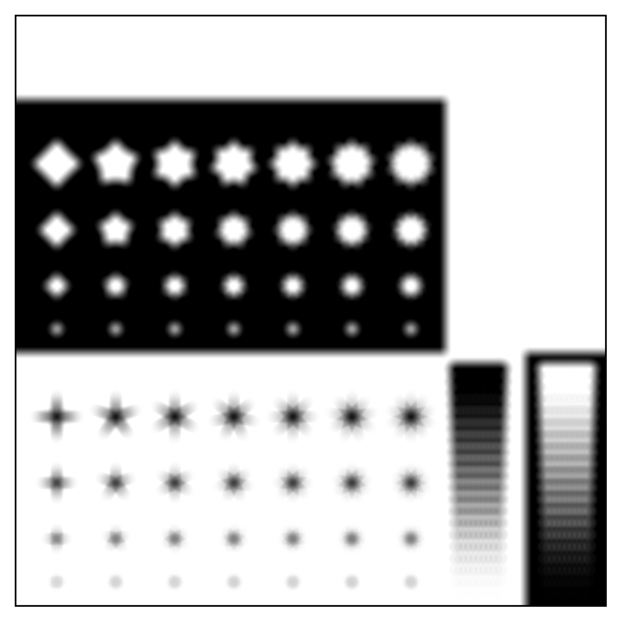
Fig. 24 Ice concentration within 15 km radius for for scene 2.

The SIT underestimation as a function of ice concentration for the radius of 15 km and 50 km is shown in Fig. 25. For small ice concentrations the underestimation for both radii is very high as expected. For 80 % ice concentration there is a strong drop in underestimation for the 50 km radius which occurs only beyond 90 % ice concentration for the 15 km radius. This is due to the fact that the 15 km radius is not enough to account for all the influence of the ice concentration on the SIT retrieval. Also note that the scene geometry influence this kind of analysis, as the shapes of the ice concentration features are not circular.

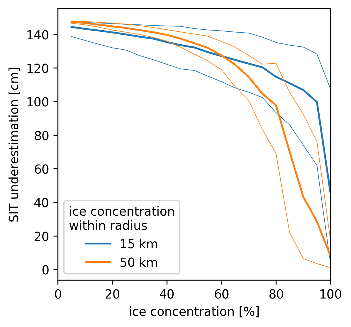
Fig. 25 SIT underestimation as a function of ice concentration for different radii around the pixel for scene 2.

Summary

The results indicate that the underestimation of SIT is significantly influenced by ice concentration and the radius used for analysis, highlighting the importance of high sea ice concentration for an accurate retrieval of SIT. The findings suggest that a larger radius may be necessary to capture the full impact of ice concentration on SIT measurements, particularly in regions with varying ice distribution. The actual sea ice concentration is not part of this processing, so that its influence can not be considered here as SIT uncertainty. This analysis underscores the need for incorporating actual sea ice concentration data in future studies to better understand and quantify the uncertainties associated with SIT retrievals. Additionally, it highlights the potential for improving retrieval algorithms by integrating spatial information about ice concentration and its variability, which could lead to more accurate assessments of sea ice thickness in diverse environmental conditions.